Summary

The concepts of momentum and impulse are addressed. The focus is on how the impulse is equal to a change in momentum which can be determined either by direct knowledge of the initial and final momentum states or by knowing the net force applied over time.

Atomistic Goals

Students will be able to...

1. Determine the magnitude of the momentum for various objects.
2. Conclude that momentum is a vector because it is the product of a vector and a scalar. 
3. Determine the momentum of a system including multiple objects.
4. Demonstrate it is harder to stop an object with larger momentum.
5. Recognize that the impulse-momentum theorem can be derived from Newton's 2nd and 3rd laws.
6. Define impulse as the change in momentum or equivalently as the average net force multiplied by the time elapsed during the interaction. 
7. Determine the change in momentum using the appropriate vector operation diagram.
8. Determine the change in momentum using the mathematic representation. 
9. Show that impulse is equal to the area under a net force as a function of time curve.
10. Identify that for a system with two objects where the net external force is zero, the impulse on one is equal and opposite of other because of
11. Newton's 3rd law, and thus the net impulse of the system is zero.
12. Recognize that impulse, change in momentum, net force, acceleration, and change in velocity are all vectors that point in the same direction.
13. Use Newton's 3rd law to show that the contribution of the impulse from one object is negative the impulse from another object during the interaction between the two.

Average Quantities | Position and Displacement

You can define a position vector by it's x and y components.

$\overrightarrow{r}=\langle x, y \rangle$

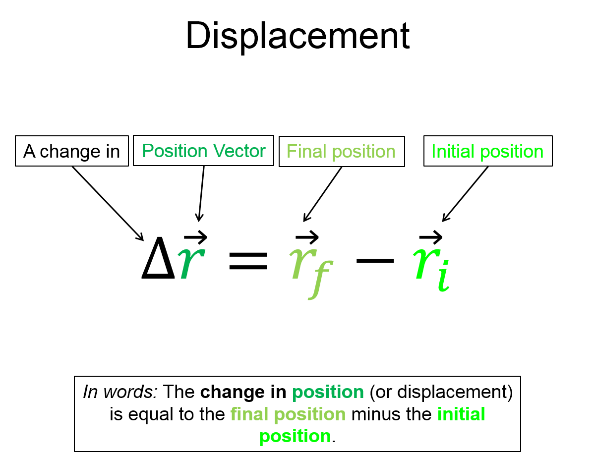
You can also define the change in position (or displacement) as the final position minus the initial position.

$\Delta \overrightarrow{r}=\overrightarrow{r}_f - \overrightarrow{r}_i$

The vector diagram for a situation like this is below. In the case of position vectors, it is also what a birds-eye view might see. The axis, with origin o, defines the point <0, 0> and the positive $\hat{x}$ and positive $\hat{y}$ directions. (Note: the symbol $\hat{x}$ is called x hat and can be thought of as a way to show which direction is the positive x direction. It is technically a unit vector but that formality is unnecessary at this point.) You could imagine an object that begins at point q and after some time, ends at point p. The change in position, labeled $\Delta \overrightarrow{r}_{qp}$ points from the initial position q, to the final position p.

The first important feature of the above diagram is that the position vector $\overrightarrow{r}_q$ can be added to the change in position vector $\Delta \overrightarrow{r}_{qp}$ using the head to tail method. The vectors don't even have to be transposed because they are already setup in the correct orientation. The resultant of that addition would be the vector $\overrightarrow{r}_{p}$. The next lesson is that you can now do regular algebra on that expression and solve for any of the vectors. The change in position $\Delta \overrightarrow{r}_{qp}$ has been derived above. The expression could also have been algebraically manipulated to solve for $\overrightarrow{r}_q$ in terms of the other two. For more algebraic rules regarding vector equations, see BoxSand's pre-lecture videos.

The term Average here refers to the fact that we are only concerned with snapshots in time and the object didn't necessarily travel along the change in position vector direction. It could have followed a curved path because all we know is that it was initially in one location and is now in another. So this could be referred to as the average change in position, but we just call it the change in position.

Average velocity is just a small step away from change in position.

$\overrightarrow{v}_{average}=\frac{\Delta\overrightarrow{r}}{\Delta t}$

Here $\Delta t$ is the change in time from the initial to final position. It's important to note that when a vector quantity, such as $\overrightarrow{v}_{average}$ is set equal to another vector quantity, such as $\Delta\overrightarrow{r}$, and the only other quantity in the relationship is a scalar, such as $\frac{1}{\Delta t}$, then both vector quantities must point in the same direction. So $\overrightarrow{v}_{average}$ points the same direction as $\Delta\overrightarrow{r}$. You can also apply the same algebraic rules to this equation and solve for any of the quantities.

To see how this looks when analyzing the average acceleration, see the pre-lecture videos below.

OpenStax is a great, free online textbook that we will use throughout this site. This section covers Position and Displacement.

OpenStax: This section covers Time, Velocity, and Speed.

OpenStax: This section covers Acceleration.

Position and Displacement

Position Vector (LB) (3 min)        

Displacement Vector (LB) (5 min)        

Additional Suggested BoxSand Videos

Displacement example (7 min) - @ the 7:00 mark I accidentally swap x and y components which is incorrect.       

Displacement summation example (13min)        

This Khan Academy video does a great job of showing the difference between instantaneous speed, velocity, for one dimensional motion. There's a bit towards the end that involves a bit of history and a note about calculus, the video does not use that calculus though, when it does an example.

Doc Schuster has created a wonderful series on youtube to help students understand their physics. This video is a fairly in-depth example involving average velocity. This video also shows how you are not anchored to using the average velocity equation as it is given, you are free to preform any algebraic manipulation you would with any other equation.

University of Toronto sim describing difference between displacement and distance

This interactive quiz from The Physics Classroom asks you to simply name that motion. This simulation should solidify difference between average velocity and instantaneous velocity as well as the effect of acceleration on a moving object. *Note, the frame of the animation is a bit small when you first run it, you can click on the lower right corner and drag to make the animation frame larger.

For additional simulations on this subject, visit the simulations repository.

 For additional demos involving this subject, visit the demo repository

Oh no, we haven't been able to write up a history overview for this topic. If you'd like to contribute, contact the director of BoxSand, KC Walsh ([email protected]).

Oh no, we haven't been able to post any fun stuff for this topic yet. If you have any fun physics videos or webpages for this topic, send them to the director of BoxSand, KC Walsh ([email protected]).

This page from The Physics Classroom will help in determining the difference between average and instantaneous quantities, representing vector quantities, and calculated average quantities.

Another page from The Physics Classroom that helps with the same as the above, but this time focusing on Acceleration.

Hyper Physics is also another resource that will be on almost every page.  Each page on a subject is made to be a quick little note with the relevant information, making Hyper Physics a great reference page. This page for instance gives a concise reference for velocity, and average velocity.

Resource Repository

This link will take you to the repository of other content on this topic.

1. Finding the change in position, average velocity, or acceleration only involves consideration of the initial and final state of the system during that time period.
2. Knowledge of what caused a system to change its acceleration, namely the net force, will not be required in this section.
3. A coordinate system should be defined in every case but if one is not explicitly written, it will be assumed positive $\hat{x}$ is to the right and positive $\hat{y}$ is upward.

1. Read and re-read the whole problem carefully.

2. Visualize the scenario.  Mentally try to understand what the object is doing. 

a.  Motion diagrams are a great tool here for visual cues as to what the motion of an object looks like.

3. Draw a physical representation of the scenario;  include initial and final velocity vectors, acceleration vectors, position vectors, and displacement vectors.

4.  Define a coordinate system;  place the origin on the physical representation where you want the zero location of the x and y components of position.

5.  Identify and write down the knowns and unknowns.

6.  Write out the mathematical representation for the physical representation you drew in step (3).

7.  Carry out the algebraic process of solving the equation(s).

            a.  If simple, desired unknown can be directly solved for.

            b.  May have to solve for intermediate unknown to solve for desired known.

            c.  May have to solve multiple equations and multiple unknowns.

            d.  May have to refer to the geometry to create another equation.

8.  Evaluate your answer, make sure units are correct and the results are within reason.

• Remember that speed is a scalar quantity which lacks direction, and velocity is a vector quantity which includes direction
• When given multiple velocities, lets say 3 velocities, and attempting t find the average velocity, you cannot just add the velocities together and divide by three. You can find the average this way only if each velocity is traveled for the same amount of time, which will rarely be the case.

• Always ask yourself if the questions is asking for a vector or a scalar quantity.
• Always ask yourself it the information given is a vector or scalar quantity.
• Draw a physical representation for the situation. Often this includes vector operation diagram.

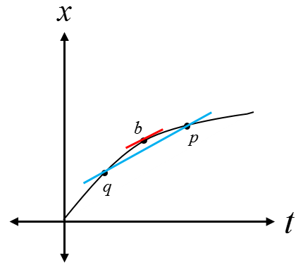
Below is a graph with position on the vertical axis and time on the horizontal. The curve shows a tangent line, or slope, representing in instantaneous velocity at one point. There is also a representation of the average slope and thus velocity between two points.

We could go out to an ordinary city block and time how long it takes to walk from one corner of the block to the exact opposite corner. In this way, we could walk around the outside of the block and measure the distance traveled on foot around the block. Each side of the block would represent a position vector. From the mathematical representation section we would certainly know what to do with the rest information. Therefore, we can easily calculate the the average velocity. 

1. A ball is set on the end of a table which is 6 meters long. The ball rolls to the other end of the table in 1 minute. What is the average velocity of the ball, in meters per second?

2. A ball is thrown straight down off a cliff with an initial downward velocity of $5 \frac{m}{s}$. It falls for 2 seconds, when the downward velocity is recorded as $24.6 \frac{m}{s}$. What is the balls average acceleration($\frac{m}{s^2}$) during that time?

3. An object moving in a straight line experiences a constant acceleration of $10 \frac{m}{s^2}$ in the same direction for 3 seconds when the velocity is recorded to be $45 \frac{m}{s}$. What was the initial velocity of the object?

CLICK HERE for solutions

BoxSand's Quantitative Practice Problems

BoxSand's Multiple Select Problems

Practice Problems: Multiple Select and Quantitative.

Recommended example practice problems 

• Set 1: 8 Problem set with solutions following each question. Be sure to try to question before looking at the solution! Your test scores will thank you. Website
• Set 2:  Problems 1 through 6. Website

For additional practice problems and worked examples, visit the link below. If you've found example problems that you've used please help us out and submit them to the student contributed content section.