1D Kinematics: Nuts & Bolts
1D Kinematics: Nuts & Bolts
3. Nuts & Bolts
Algorithm
Expand
- Read and re-read the whole problem carefully.
- Visualize the scenario. Mentally try to understand what the object is doing.
- Motion diagrams are a great tool here for visual cues as to what the motion of an object looks like.
- Draw a physical representation of the scenario; include initial and final velocity vectors, acceleration vectors, position vectors, and displacement vectors.
- Define a coordinate system; place the origin on the physical representation where you want the zero location of the x and y components of position.
- Identify and write down the knowns and unknowns.
- Identify and write down any connecting pieces of information.
- Determine which kinematic equation(s) will provide you with the proper ratio of equations to number of unknowns; you need at least the same number of unique equations as unknowns to be able to solve for an unknown.
- Carry out the algebraic process of solving the equation(s).
- If simple, desired unknown can be directly solved for.
- May have to solve for intermediate unknown to solve for desired known.
- May have to solve multiple equations and multiple unknowns.
- May have to refer to the geometry to create another equation.
- If multiple objects or constant acceleration stages or dimensions, there is a set of kinematic equations for each. Something will connect them.
- Evaluate your answer, make sure units are correct and the results are within reason.
Multiple Representations
Observe the different types of representations for this section below;
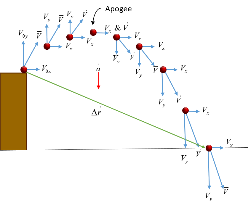
Physical Representation
Kinematics problems are often analyzed with physical descriptions. Below we have an object launched from a ledge with initial horizontal and vertical velocity components. The vectors indicate the relative magnitudes of the horizontal and vertial velocity components at different stages of the objects motion.
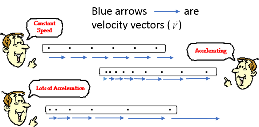
In addition, simple 1D motion diagrams are utilized to describe the speed of an object and whether or not the object has any acceleration.
Mathematical Representation
Main kinematics equations. Notice that we use $ r $ to represent the vector position. In the videos below, Professor Matt Anderson uses $ x $ and $ y $ to denote position in a given coordinate direction.
$ \vec{r}_{f} = \vec{r}_{i}+\vec{v}_{i} \Delta t + \frac{1}{2} \vec{a} \Delta t^{2} $
$ \vec{v}_{f} = \vec{v}_{i} + \vec{a} \Delta t $
$ v_{fx}^{2} = v_{ix}^{2}+2a_{x} \Delta x $
Watch Professor Matt Anderson explain 1D and 2D Kinematics equations using the mathematical representation.
Video 1: Kinematics equations in 1D
Video 2: Kinematics equations in 2D
Graphical Representation
the Physics Classroom introduces the relationship between kinematics equations and their graphical representation. In addition, for a more indepth discussion please refer to the graphical anaysis section.
![]()
Descriptive Representation
The branch of mechanics concerned with the motion of objects without reference to the forces that cause the motion.
Actual Representation
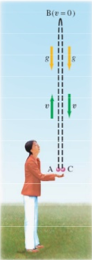
For example, a person throws a ball upward into the air with an initial velocity of $15.0 \frac{m}{s}$. You can calculate how high it goes and how long the ball is in the air before it comes back to your hand. Ignore air resistance.
Example Problems
Set 1: RedKnightPhysics, Problems 1-16
Set 2: Hyperphysics motion examples
For additional practice problems and worked examples, go here.