All of the lessons learned while practicing linear kinematic problems are relevant when solving rotational kinematic problems.

1. Visualize the motion of the object(s) in question.

2. Identify your system - this can be aided by drawing a dotted line around your system.

3. Draw a physical representation. A physical representation is not just a pretty picture but rather a simple figure that includes a representation of important physical quantities such as angular velocity. The diagram should include a representation of initial and final angular velocity, angular acceleration, change in angle, and (sometimes) time. An example for an object slowing down is below.

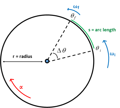
4. Identify known and unknown quantities. That means for each stage/object in the system there are five kinematic quantities ($\Delta \theta, \omega_i, \omega_f, \alpha, t$ to put in a known or unknown category. Follow the convention of CCW being positive for the sign of each quantity. For example in the above figure, the initial and final angular velocities are in the CCW direction and thus would be positive. The angular acceleration though, since the object is slowing down, points in the opposite direction as the velocity and thus is CW and would be a negative number.

5. Use the kinematic equations of constant acceleration to solve for the unknown quantities.

(i)   $\Delta \theta = \omega_i \Delta t + \frac{1}{2} \alpha \Delta t^2$

(ii)   $\omega_f = \omega_i + \alpha \Delta t$

(iii)   $\omega_f^2 = \omega_i^2 + 2 \alpha \Delta \theta$

This may require solving simultaneous equations. One way to approach this step is to find the same number of equations as number of unknowns. It then mathematically can be solved.

6. Lastly, and especially if you get stuck in part 5, remember there are connections between the angular and linear kinematic variables. This may be used to give you a new equation with no new unknowns or to simply change your answer from an angular to linear value. An example might be after finding the object subtended 2 Rads, you convert that to the distance it traveled in meters. Use the connections between the linear and angular variables below.

Change in angular position ==> Distance traveled:   $s=\Delta \theta r$

Angular velocity ==> speed:   $|\overrightarrow{v}| = v_t = \omega r$

Angular acceleration ==> Tangential component of linear acceleration:   $a_t = \alpha r$

$\overrightarrow{v}=\langle v_r, v_t, v_z \rangle = \langle 0, \omega r, 0 \rangle$

$\overrightarrow{a}=\langle a_r, a_t, a_z \rangle = \langle \frac{v^2}{r}, \alpha r, 0 \rangle$

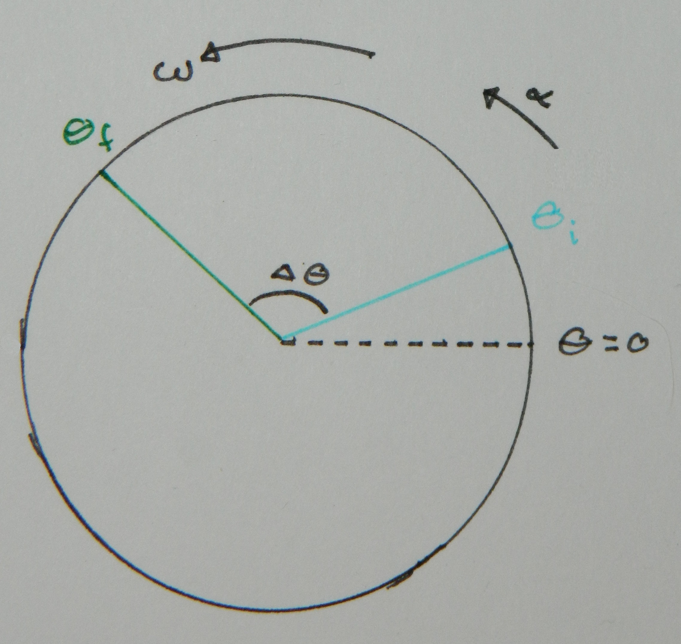
$\theta$ is the angular position, $\omega$ is the angular velocity, $\alpha$ is the angular acceleration. 

$\Delta \theta = \omega_i \Delta t + \frac{1}{2} \alpha \Delta t^2$
$\omega_f = \omega_i + \alpha \Delta t$
$\omega_f ^2 = \omega_i^2 + 2\alpha \Delta \theta$

The relations between angular and linear,
$S = \Delta \theta r $, $v_{\text{tangential}} = \omega r$, $a_{\text{tangential}} = \alpha r$

Angular frequency ($\omega$), Angular acceleration ($\alpha$)

Below is the plot of the angular position ($\theta$) as a function of time for some object increasing its speed will traveling in a circle.

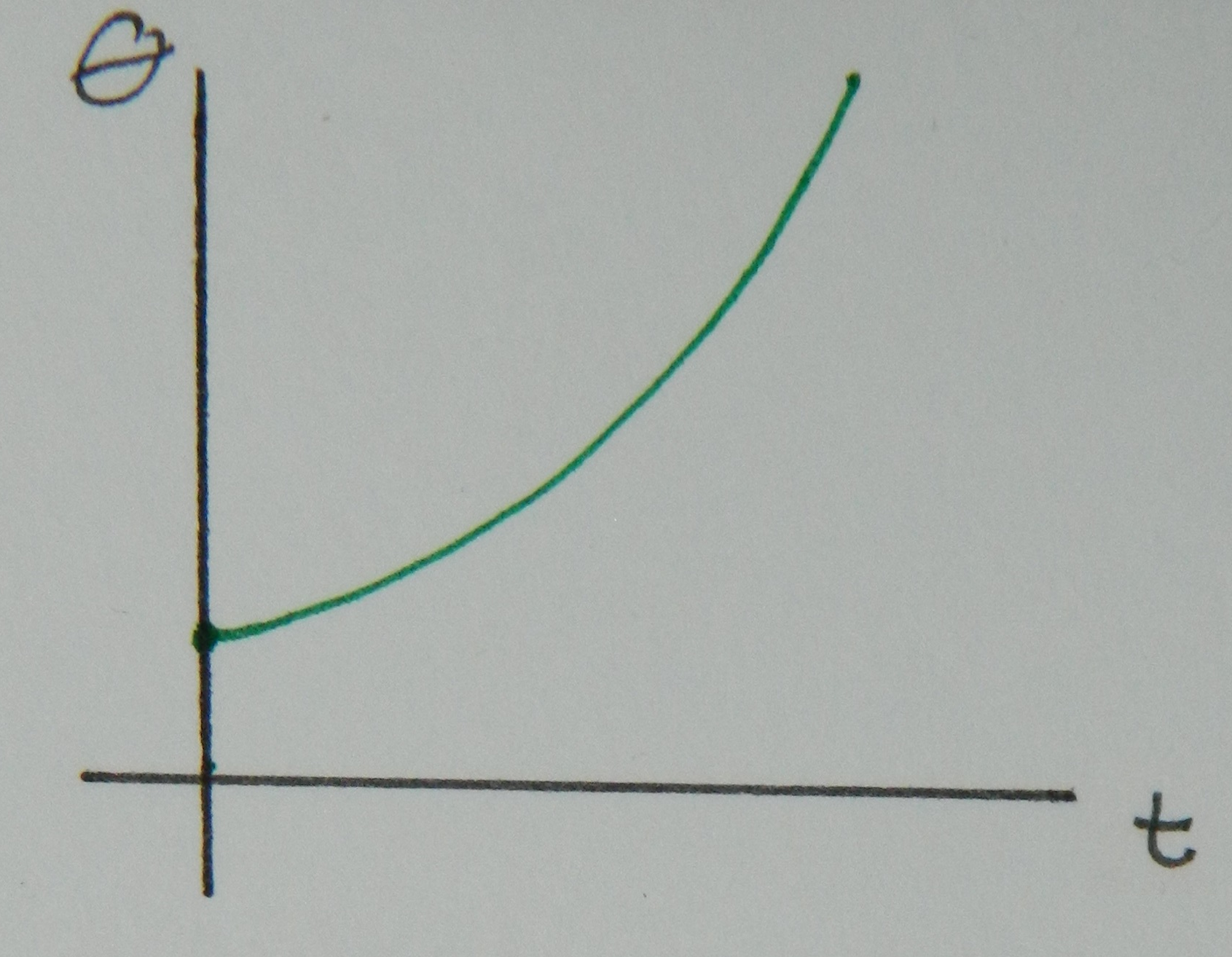
The slope of the position plot, this time measured as an angle, with respect to time is equal to the angular velocity ($\omega$). This is no different than in linear motion where velocity is the slope of position. Since the slope of the angular position as a function of time is increasing, that behavior is displayed in in the angular velocity as a function of time below.

$\omega = \frac{\Delta \theta}{\Delta t}$

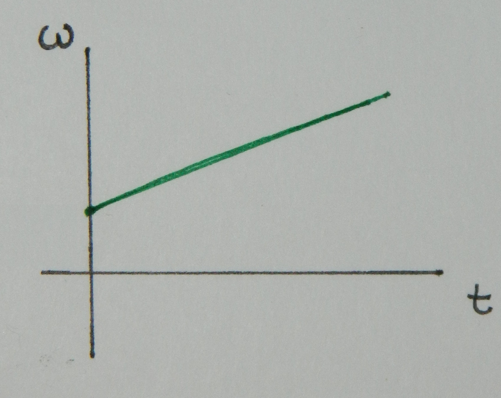
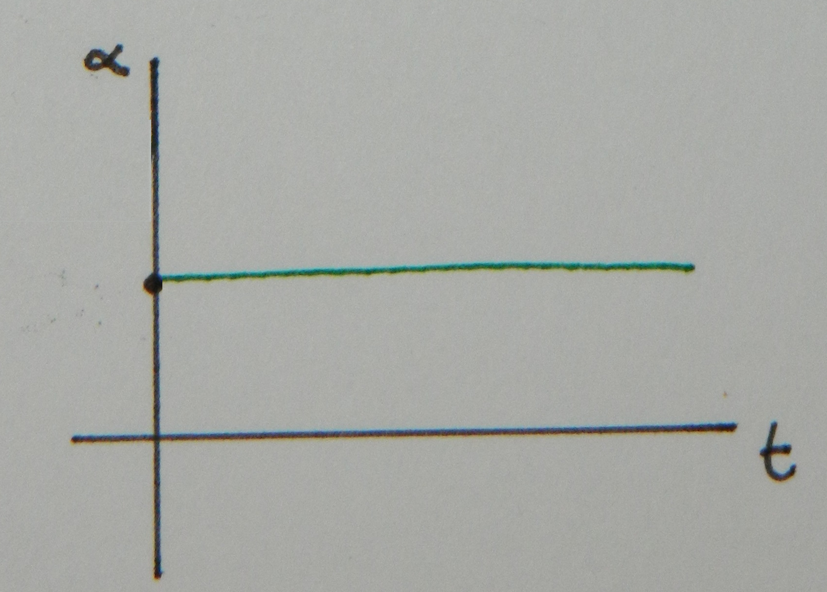
The angular acceleration ($\alpha$) is the slope of the angular velocity. Since the slope of the above plot is constant, the value of the angular acceleration is a constant, as shown below.

$\alpha = \frac{\Delta \omega}{\Delta t}$

This is analogous to the linear position, velocity, and acceleration graphs, which means that to go the other way, like from acceleration to velocity, you'd use the area under the plot.

At $t_i$ a disk is spinning with an angular velocity of $\omega_i$, with an angular acceleration of $\alpha$. After t seconds the disk has and angular velocity of $\omega_f$, and has experienced a change in angular position $\Delta \theta = \omega_i \Delta t + \frac{1}{2} \alpha \Delta t^2$. 

You can setup an experiment to study the phenomena of constant angular acceleration. An example is demonstrated below.