BoxSand's Resources
Introduction
Lets recall the concept of a field.
Things create fields that alter the space around them in such a way that facilitates interactions with other things. The field is owned by the original thing and in that way precludes the existence of the second thing and any interactions that may occur between the two.
We've learned about how the electric field can be used to describe force interactions. The concept is that the first charged particle $A$ creates an electric field $\overrightarrow{E}_{A}$ that the second test charged particle $O$ resides in. Particle $O$ then feels a force $\overrightarrow{F_O}$ equal to the charge of $O$ ($q_O$), multiplied by the electric field of $A$.
$\overrightarrow{F}_O=q_O \overrightarrow{E}_A$
The electric potential $V$ is connected the electric potential energy $U$ in a similar way. The electric potential is the field created by charge $A$ that test charge $q_O$ resides in. The potential energy of the system is then the charge $q_O$, multiplied by the electric potential from $A$.
$U_{OA} = q_O V_A$
Recall that energy is a scalar quantity and so is the charge of a particle. That means that the electric potential $V$ must also be a scalar. The electric potential is a scalar field, it's a number at every point in space. It is used to describe how a charged particle alters the space around them (in an abstract way) and is used to quantify the potential energy between the charge originating the field and those residing in the field. Pulling from the example in the Overview, we know that if two protons are next to each other they will repel one another and speed up. They will increase their kinetic energy as they both move towards the state with a minimum of potential energy, a state far away from each other. This is all due to the interaction between them - the electric potential is the field we use to describe the interaction with an energy analysis.
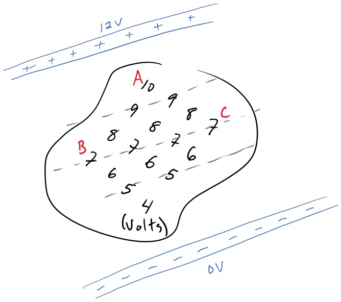
To get a better feel for how the electric potential works, lets think about fields as a map. Below is an example of an electric potential field from some group of charges that are not shown in the figure. For now don't be concerned with how the charges created this particular field, we will cover field patterns from charge distributions shortly. Instead concentrate on how the energy of a charged particle in an electric field can be analyzed. Remember that the electric potential is a scalar field and as such is just a number everywhere in space. For the electric potential it is measured in volts, the same volts you're used to with batteries and electronics. The field is there before the positive charge shown even exists.
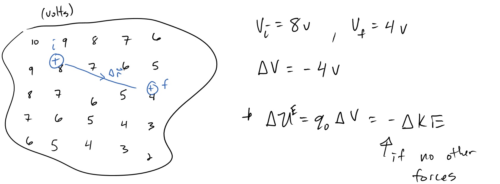
Now imagine the positive charge $q_O$ is initially at a location where the electric potential is 8 Volts. That means it has an electric potential energy at that location is $U_{initial}=(8 volts)(q_O)$, where $q_O$ is in SI units of Coulombs. If the positive charge $q_0$ was to move though the displacement $\Delta \overrightarrow{r}$ to the final location, it will have decreased in electric potential energy. The electric potential at the final location is 4 Volts and thus the electric potential energy is $U_{final}=(4 volts)(q_O)$. The potential energy has decreased and so, barring no other interactions, the kinetic energy must increase. This does lead to an important conclusion.
Positive charges feel a force and speed up in the direction of decreased electric potential.
It's because that decreases the electric potential energy. All particles feel a force in the direction of decreased potential energy, but be careful, for a negative charge, it feels a force toward increased electric potential because that actually decreases the electric potential energy. The minus sign on the charge accounts for the difference between the positive charge moving towards decreased potential while the negative charge moves towards increased potential. Both do so to decrease the potential energy.
This example also illustrates the power of the field concept. Once we have found the electric potential field from a charge distribution, we can perform an infinite number of theoretical experiments on how much energy is converted between kinetic and potential for of any charge moving between locations in space. To make it more tangible, lets connect to the analogy of the gravitational field and gravitational potential energy. Recall that gravitational potential energy $U^g = mgh$. The gravitational field is equal to $gh$ and when multiplied by the mass you get the gravitational potential energy $mgh$. Since $g$ is a constant, the field really only depends on your height (or elevation). A topographical map is essentially a gravitational potential map.
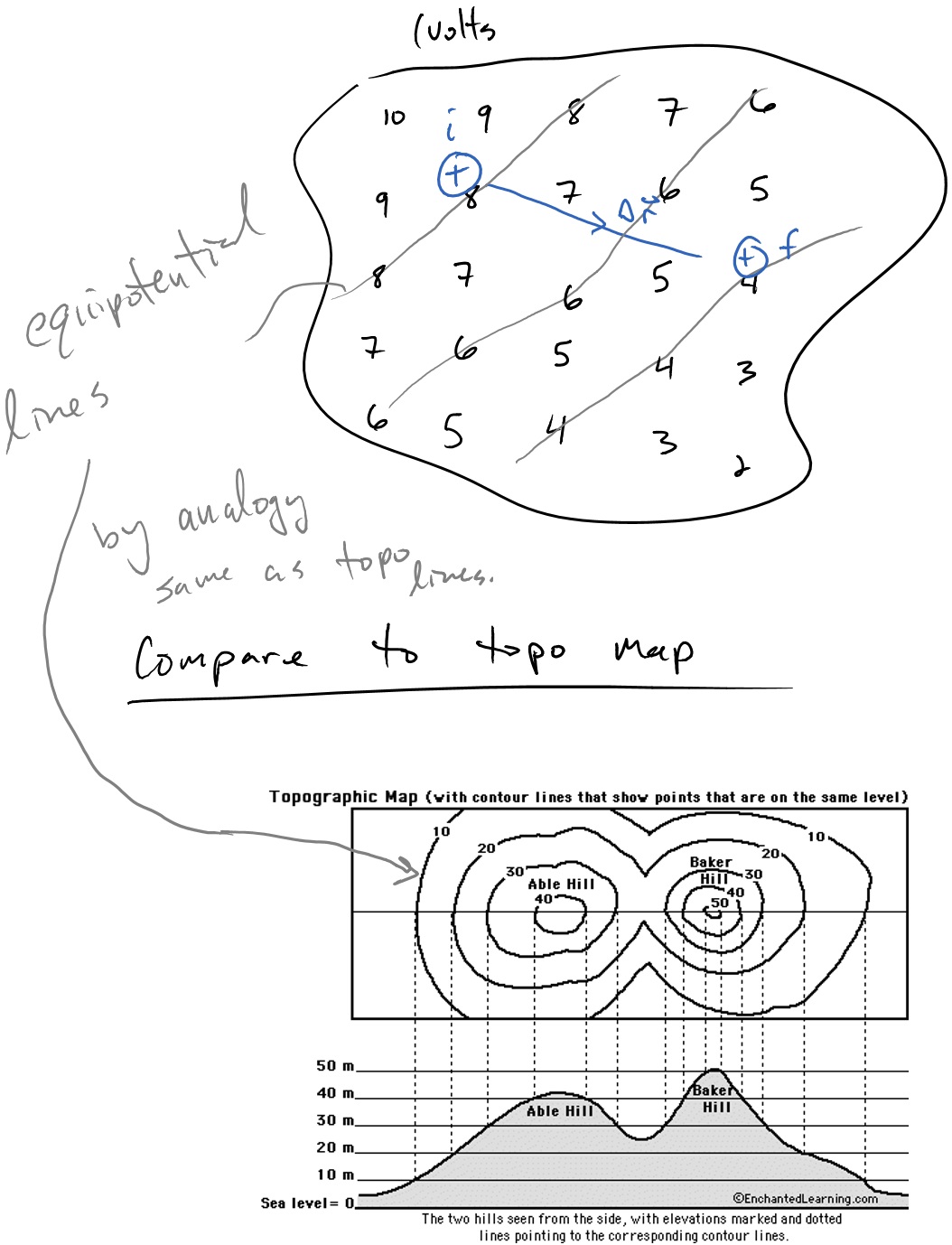
Lines (or really surfaces) called equipotentials can be used to describe places that have a constant potential and thus energy. Masses feel a force that make them want to move down the equipotentials, analogous to the positive charge above feeling a force towards decreased electric potential. In both cases (charges and masses) the systems move towards decreased potential energy. This is one of the most fundamental statements that can be made in physics - systems drive towards decreased potential energy. This is why water runs downhill.
Electric Potential from Point Charges
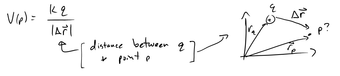
Most charge distributions are not that of point charge but they are comprised of the electric potential from each individual particle making up the charge distribution. Think a charged plate is sheet of point charges. To understand how a collection of charges creates a field, lets first look at how each individual point particle creates a field. The electric potential of a point charge $q$ is equal to:
$V=\frac{kq}{r}$, where r is the distance from the point charge and k is a constant.
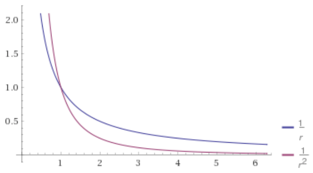
The first thing to note is that the electric potential $V$ decreases like $\frac{1}{r}$ as opposed to the electric field magnitude that falls off like $\frac{1}{r^2}$. The potential decreases more slowly than the electric field strength. This can be seen by comparing the nature of each function in the graph below where $\frac{1}{r}$ gets smaller more rapidly than $\frac{1}{r^2}$.
Another difference is the electric field is a vector field while the electric potential is a scalar field. That is very good news when it comes to calculations as it's much easier to deal with a bunch of numbers than it is to deal with a bunch of vectors - the mathematics are more simple. The below equation is more rigorous than the one above and it reads: the electric potential at point p is equal to the constant $k = \frac{1}{4\pi \epsilon{0}}$, multiplied by the charge $q$, and divided by the absolute value of the displacement between the charge $q$ and the point p.
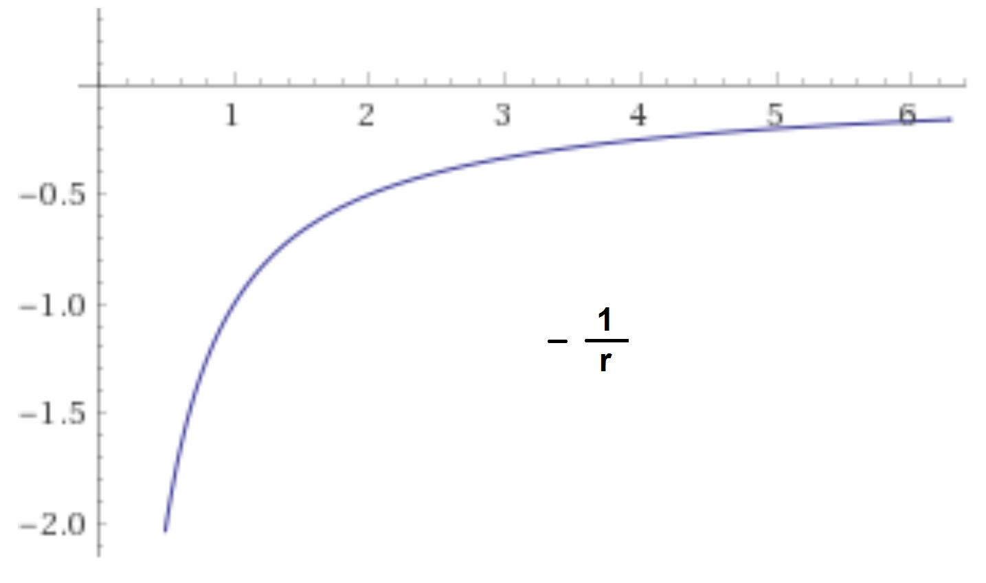
When performing calculations of the field you get a number, positive for positive charges and negative for negative charges, for every point in space. The graph of the electric potential from a positive charge is the $\frac{1}{r}$ above while the negative sign for a negative makes the graph for a negative charge as a function of distance proportional to $-\frac{1}{r}$. Below is a graph of $-\frac{1}{r}$ to show the nature of the function.
Electric Potential for Charge Distributions
The electric potential field from a single charged particle $q$ is above. To find the field from a group of charges you can simply add up the contributions from each individual particle at the location of interest. Potentials add through the principle of superposition, which means you just add them up with no other scaling factors.
$V_{total}(p) = \Sigma V_i(p) = V_1(p) + V_2(p) + ...$
An example of a charge distribution is a set of parallel charged plates. Take two metal sheets and charge one of them positively and the other negatively. This creates an electric potential between them, after all if you put an electron or proton in between them they would both speed up, albeit in opposite direction. The 2-D figure below depicts the voltage (electric potential) in the region between the two plates. The 3-D graph uses the third (vertical) axis to describe the voltage, whereas 2-D represents it as a number.
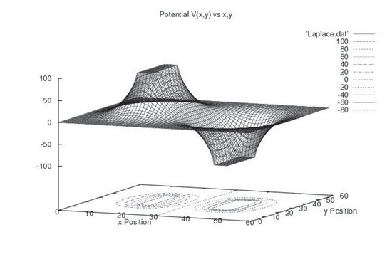
Both figures show the equipotentials, with the 3-D projecting them onto the floor of the graph.
Connecting the Electric Potential and the Electric Field
The electric field and potential have a close relationship. In 1-D the electric field can be thought as negative the slope of the electric potential.
$\bar{E}_x = -\frac{\Delta V}{\Delta x}$
Lessons from the above equation are:
1) if $\frac{\Delta V}{\Delta x} = constant$ (linear), then $E_x$ is constant and uniform, this is the case near large sheets of charge and in parallel plate capacitors.
2) The relationship between the electric field and potential is independent of the test charge $q_0$ - it's independent of other charges interacting with the field
3) The minus sign tells us the electric field points towards decreasing electric potential - if $\frac{\Delta V}{\Delta x}$ is negative, $E_x$ is positive
In 3-D the electric field is negative the gradient of the electric potential.
$\overrightarrow{E} = - \langle \frac{\Delta V}{\Delta x}, \frac{\Delta V}{\Delta y}, \frac{\Delta V}{\Delta z} \rangle$
A gradient is a vector and can be thought of as a kind of 3-D slope that points in the direction of steepest ascent. With the minus sign the electric field points in the direction of steepest descent. Since this is the direction of the force on a positive charge we can again make the analogous connection to the gravitational field and how water is forced to run downhill, down the direction of steepest descent. This feature adds one more lesson:
4) The electric field is perpendicular to equipotential surfaces and lines
Total Potential Energy of a Collection of Particles
One question that often arises is what is the total electric potential energy of a collection of particles. Imagine a single positive charge fixed in space. To bring a second charge close to the first, you'd have to do work to overcome the repelling force. If you did overcome that work and brought them next to each other, if they were released, they would fly away with kinetic energy. That kinetic energy comes originally from the work of bringing them together, which is converted into potential energy when they are close together. That potential energy can be thought of as the energy of the system. If you where to bring in more charges, you'd have to figure out the potential energy of all the combinations particles. The total potential energy for a system of three particles is described below.
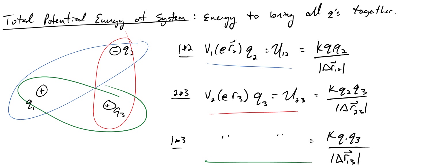
The total potential energy of the system of three particles is just summation of all the combinations. *Warning* don't over count interactions, $U_{12}$ is the total energy of the 1 and 2 system, meaning if you were to also include $U_{21}$, you'd be double counting. So it's only the unique pairs and the ordering of the subscripts does not matter.
$U_{total}=U_{12} + U_{23} +U_{13}$ ... + all combinations if there are more particles
This is how much energy would be released into kinetic energy if the system was released from rest. Notice that if there were negative charges present you could have a negative total potential energy. Systems with a negative potential energy are said to be bound systems as the particles have a net attraction to one another. They want to clump together as opposed to fly apart.
Summary
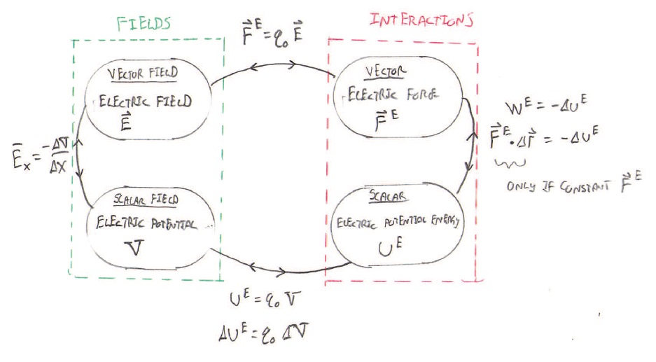
We can now go full circle with the connections between the electric field and potential, and the electric force and energy. The electric field and potential are owned by the charge distribution and preclude any interactions with new test charges $q_0$. The electric force and potential energy require an interaction with the test charge. The concept map below helps visualize the relationship.
Videos
Pre-lecture Videos
Watch these videos before doing the pre-lecture assignment. There's a lot of videos here, check the daily learning guide to know which videos are needed for which lecture. We've also broken grouped the links by day, because we're nice people. ** denotes supplemental but suggested
E-potential energy from conservative work(11min)
E-potential energy from conservative work(11min)
E-potential - example - energy from conservative work(5min) **
E-potential - example - energy from conservative work(5min)
E-potential - conservative work proof(5min) **
E-potential - conservative work proof(5min)
E-potential from EPE(8min)
E-potential and the concept of map(5min)
E-potential and the concept of map(5min)
Field philosophy(4min)
E-potential - example - energy from potential(5min) **
E-potential - example - energy from potential(5min)
E-potential - review connecting to topo maps(1min) **
E-potential - review connecting to topo maps(1min)
E-potential - e fields and interactions concept map(7min) **
E-potential - e fields and interactions concept map(7min)
E-potential - conservation of energy from map and plot(7min) **
E-potential - conservation of energy from map and plot(7min)
E-potential and E-field connection for uniform field(9min)
E-potential and E-field connection for uniform field(9min)
E-potential and E-field connection for nonuniform field(5min)
E-potential and E-field connection for nonuniform field(5min)
E-potential and E-field connection - 3D gradient(2min)
E-potential and E-field connection - 3D gradient(2min)
E-potential and work nonuniform field(3min)
E-potential and work nonuniform field(3min)
E-potential from point charges(4min)
E-potential from point charges(4min)
E-potential from point charges example(4min)
E-potential from point charges example(4min)
E-potential and EPE plotted for point charges(4min)
E-potential and EPE plotted for point charges(4min)
E-potential from point charges example_energy(6min)
E-potential from point charges example_energy(6min)
E-potential energy of a system of charges(8min)
E-potential energy of a system of charges(8min)
E-potential dielectric breakdown(7min)
E-potential dielectric breakdown(7min)
Web Resources
Text
Openstax has five relevant sections covering the electric potential.
| Introduction to Electric Potential | Electric Potential Energy | Electric Potential in a Uniform Electric Field |
| Electric Potential Due to a Point Charge | Equipotential Lines |
The Physics Classroom has two sections for us, one on electric potential and the other on electric potential difference.
| Electric Potential | Electric Potential Difference |
Boston University's Page on electric potential is a neat reference with a couple of example problems
![]()
PPLATO is a complete resource with a lot of information, and several practice questions per subject. This webpage covers electric charge, the electric field, and electric potential, we've already covered charge, and the electric field, so now it's time to focus on electric potential!
![]()
![]()
Isaac Physics' section on the electric field is a good short resource. This page contains previously studied material on electric fields as well as information on electric potential, and the connection between electric field and electric potential.
![]()
Other Resources
This link will take you to the repository of other content related resources .
![]()
Videos
Pre-Med Academy has a lot of videos about the Electric Field and Force, too many to list here. We really recommend checking out the content repository for this section and check out the rest of their videos Here are just a few on Work and Potential Energy, Electric Potential Difference, and Potential of a Point Charge
Youtube: Pre-Med Academy - Work and Potential Energy
Youtube: Pre-Med Academy - Electric Potential Difference
Youtube: Pre-Med Academy - Potential of a point charge
Step By Step Science has a bunch of practice problems having to do with electric potential and we suggest you check out your content repository for this section to see a list of relevant videos from them. Here are a few on work done moving a point charge through a potential difference, calculating potential difference between two points, and work to bring in a charge from infinity.
Youtube: Step by Step Science - charge through potential
Youtube: Step by Step Science - potential difference
Youtube: Step by Step Science - charge from infinity
Other Resources
This link will take you to the repository of other content related resources .
![]()
Simulations
This flashphysics applet lets you create charge distributions from point charges and plot the corresponding equipotential lines. Try placing test charges in the region of space to watch possible trajectories!
This PhET interactive combines electric fields, electric potential and charge (known collectively as electrostatics). Place charges around and observe the resulting electric and potential fields.
![]()
For additional simulations on this subject, visit the simulations repository.
![]()
Demos
For additional demos involving this subject, visit the demo repository
![]()
Practice
Fundamental examples
1. Two plates of metal with uniform charge distribution are held a distance d apart from each other as shown in the figure below. The metal plate on the left side is positively charged while the metal plate on the right is negatively charged.
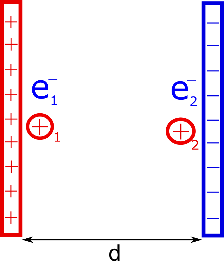
a. Which plate is considered to be at a higher potential ($V$)?
b. The electron labeled $1$ is placed in-between the two sheets as shown. Does this electron have a high or low electric potential energy? Ignore the other charges in-between the plates.
c. The electron labeled $2$ is placed in-between the two sheets as shown. Does this electron have a high or low electric potential energy? Ignore the other charges in-between the plates.
d. The proton labeled $1$ is placed in-between the two sheets as shown. Does this proton have a high or low electric potential energy? Ignore the other charges in-between the plates.
e. The proton labeled $2$ is placed in-between the two sheets as shown. Does this proton have a high or low electric potential energy? Ignore the other charges in-between the plates.
2. Two parallel plates are held $20.0 \, mm$ apart and the potential difference between the plates is $110 \, V$.
a. What is the magnitude of the electric field between the two parallel plates?
b. Which direction does the electric field point if the plate on the left has a uniform negative charge distribution and the plate on the right has a uniform positive charge distribution?
c. Sketch a physical representation of this problem. Include a few equipotential lines between the two parallel plates.
3. Two uniformly charged parallel plates are held some distance “$d$” apart from each other with an electric potential of $300 \, V$ between them. An electron is placed at rest near the negative charged plate. Calculate the speed at which the electron will hit the positive plate.
4. The figure below shows a charge distribution made up of $3$ point charges. The charges are fixed in space and cannot move. Let $q = 1 \, \mu C$ and $L = 1.0 \, cm$.
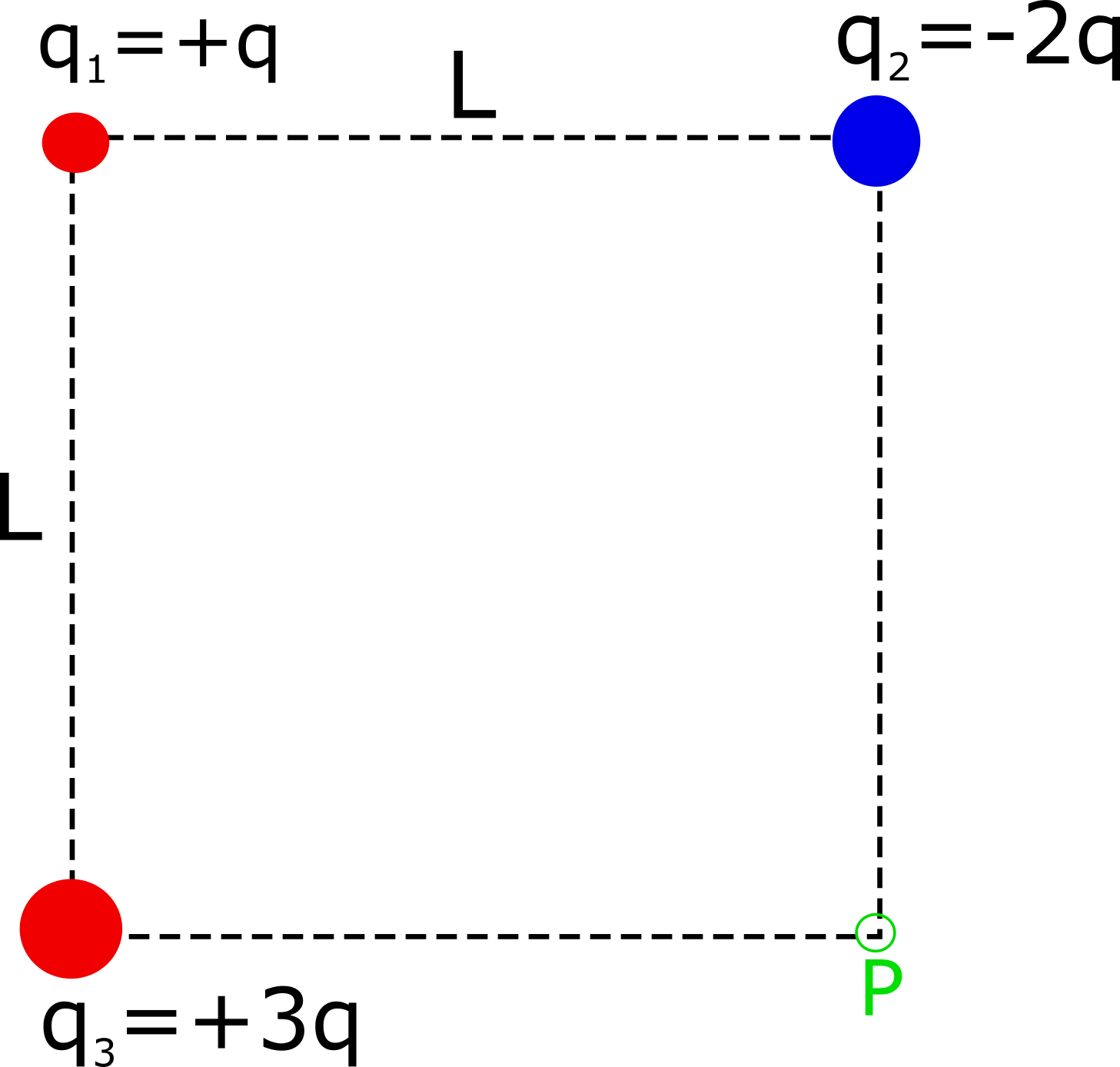
a. Find the electric potential energy of this charge distribution.
b. Find the electric potential at point P.
CLICK HERE for solutions.
Short foundation building questions, often used as clicker questions, can be found in the clicker questions repository for this subject.
![]()
Practice Problems
BoxSand practice problems - Answers
BoxSand's multiple select problems
BoxSand's quantitative problems
Recommended example practice problems
- OpenStax and it's 4 related sections. Problems at bottom of page,
- Electric Potential Energy, Website Link
- Electric Potential in a Uniform Electric Field, Website Link
- Electric Potential Due to a Point Charge, Website Link
- Equipotential Lines, Website Link
- Physics-Prep
- Electric Potential, Website Link
- Electric Potential Due to Point Charges, Website Link
- Equipotential Surfaces, Website Link
For additional practice problems and worked examples, visit the link below. If you've found example problems that you've used please help us out and submit them to the student contributed content section.
![]()
![]()