This lecture will focus on how to solve the problems introduced in the previous lecture. Today will be an opportunity to flex problem-solving muscles: a major reason for taking physics and a skill to apply to any field of study. Ask questions and make as many mistakes as possible, as this is as low-stakes as it gets (compared to homework, exams, and your future job).
Flipping Physics covers 1D Kinematics with some examples (refers to the subject as Uniformly accelerating motion).
https://media.oregonstate.edu/media/t/1_2tjds0oz
Pre-lecture Study Resources
Read the BoxSand Introduction and watch the pre-lecture videos before doing the pre-lecture homework or attending class. If you have time, or would like more preparation, please read the OpenStax textbook and/or try the fundamental examples provided below.
BoxSand Introduction
1-D Kinematics | Problem Solving Strategies
This module does not have new material but rather is focused on application of problem solving in kinematics. If you have not checked out the Problem Solving Guide, located further down on this page, I suggest you take a look. Here is the Checklist of things to consider when analyzing kinematics situations from the Problem Solving Guide.
- Read and re-read the whole problem carefully.
- Visualize the scenario. Mentally try to understand what the object is doing.
- Motion diagrams are a great tool here for visual cues as to what the motion of an object looks like.
- Draw a physical representation of the scenario; include initial and final velocity vectors, acceleration vectors, position vectors, and displacement vectors.
- Define a coordinate system; place the origin on the physical representation where you want the zero location of the x and y components of position.
- Identify and write down the knowns and unknowns.
- Identify and write down any connecting pieces of information.
- Determine which kinematic equation(s) will provide you with the proper ratio of equations to number of unknowns; you need at least the same number of unique equations as unknowns to be able to solve for an unknown.
- Carry out the algebraic process of solving the equation(s).
- If simple, desired unknown can be directly solved for.
- May have to solve for intermediate unknown to solve for desired known.
- May have to solve multiple equations and multiple unknowns.
- May have to refer to the geometry to create another equation.
- If multiple objects or constant acceleration stages or dimensions, there is a set of kinematic equations for each. Something will connect them.
- Evaluate your answer, make sure units are correct and the results are within reason.
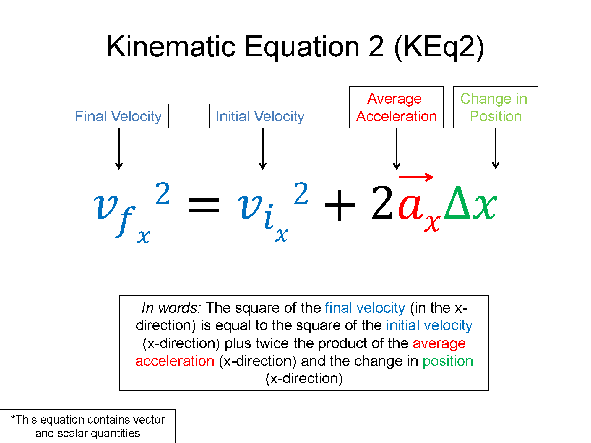
Key Equations and Infographics
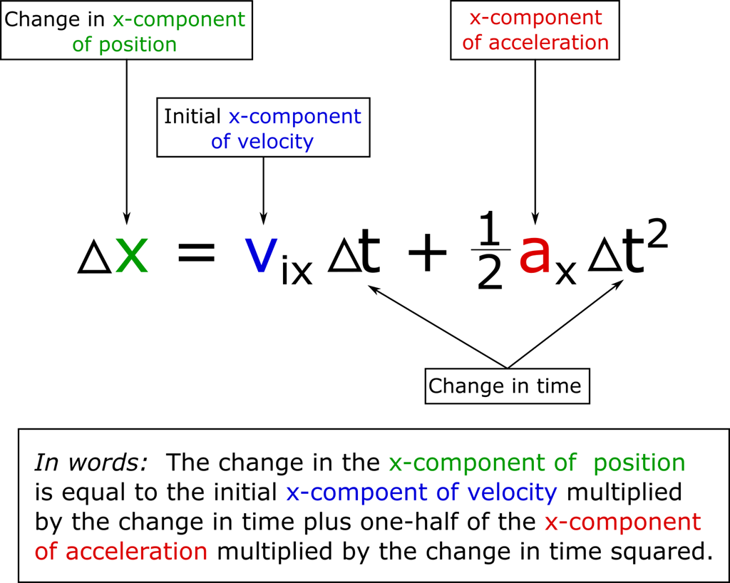
Kinematic Equation 1 (KEq1)

BoxSand Videos
Required Videos
Note how every problem is setup the same way:
Suggested Supplemental Videos
OpenStax Reading
The reading below is the same as the previous lecture.
OpenStax section 2.5 covers Motion Equations for Constant Acceleration in 1-D.
![]()
OpenStax section 2.6 covers Problem-Solving basics for 1D Kinematics.
![]()
OpenStax section 2.7 covers Falling Objects.
![]()
Fundamental examples
1. A ball is set on the end of a table which is 6 meters long. The ball rolls to the other end of the table in 1 minute. What is the average velocity of the ball, in meters per second?
2. A ball is thrown straight down off a cliff with an initial downward velocity of $5 \frac{m}{s}$. It falls for 2 seconds, when the downward velocity is recorded as $24.6 \frac{m}{s}$. What is the balls average acceleration($\frac{m}{s^2}$) during that time?
3. An object moving in a straight line experiences a constant acceleration of $10 \frac{m}{s^2}$ in the same direction for 3 seconds when the velocity is recorded to be $45 \frac{m}{s}$. What was the initial velocity of the object?
CLICK HERE for solutions
Post-Lecture Study Resources
Use the supplemental resources below to support your post-lecture study.
Practice Problems
BoxSand's Quantitative Practice Problems
BoxSand's Multiple Select Problems
Practice Problems: Multiple Select and Quantitative.
Recommended example practice problems
- Set 1: 8 Problem set with solutions following each question. Be sure to try to question before looking at the solution! Your test scores will thank you. Website
- Set 2: Problems 1 through 6. Website
For additional practice problems and worked examples, visit the link below. If you've found example problems that you've used please help us out and submit them to the student contributed content section.
![]()
Additional Boxsand Study Resources
Additional BoxSand Study Resources
Learning Objectives
Summary
The objective is to have students solve story problems involving motion along a line that require the use of multiple representations. Particular focus is on mathematical representations.
Atomistic Goals
Students will be able to...
- Identify that the motion all occurs along a line and can be treated with a 1-dimensional analysis.
- Define free-fall and identify when a free-fall analysis is appropriate.
- Denote that objects speeding up have an acceleration that points in the same direction as their velocity, while those slowing down have an acceleration that points in the opposite direction of their velocity.
- Translate a descriptive representation to an appropriate physical representation that includes a displacement vector, initial and final velocity vectors, an acceleration vector, and a coordinate system.
- Draw an appropriate physical representation for a system that includes multiple stages or objects by including vector representations for each.
- Identify known and unknown quantities for each stage or object.
- Translate from the mathematical, physical, or descriptive representation to the graphical representation.
- Translate to the mathematical representation with the help of the descriptive, physical, and graphical representations.
- Identify the appropriate kinematic equation for constant acceleration to use when analyzing the problem.
- Use one of the kinematic equations to find the value of an unknown, then use that value and another kinematic equation to solve for desired unknown.
- Solve simultaneous equations when there are two or more equations with the same two unknowns.
- Solve problems that involve multiple objects or multiple stages.
- Apply any connections between stages or objects when appropriate, e.g. the geometric connection between two runners when they do not start at the same location.
- Apply sign sense-making procedures to check their solutions.
- Apply order of magnitude sense-making procedures to check their solutions.
- Apply dimensional analysis sense-making procedures to check their solutions.
YouTube Videos
This Khan Academy video helps show how to pick which kinematic equation to use in different situations
Flipping Physics video reviewing kinematics with some problem solving strategies.
Simulations
This interactive quiz from The Physics Classroom asks you to simply name that motion. This simulation should solidify difference between average velocity and instantaneous velocity as well as the effect of acceleration on a moving object. *Note, the frame of the animation is a bit small when you first run it, you can click on the lower right corner and drag to make the animation frame larger.
![]()
For additional simulations on this subject, visit the simulations repository.
![]()
Demos
Here are some solved problems and walkthroughs
For additional demos involving this subject, visit the demo repository
![]()
History
Oh no, we haven't been able to write up a history overview for this topic. If you'd like to contribute, contact the director of BoxSand, KC Walsh (walshke@oregonstate.edu).
Physics Fun
Oh no, we haven't been able to post any fun stuff for this topic yet. If you have any fun physics videos or webpages for this topic, send them to the director of BoxSand, KC Walsh (walshke@oregonstate.edu).
Other Resources
This page from The Physics Classroom will help in determining the difference between average and instantaneous quantities, representing vector quantities, and calculated average quantities.
![]()
Another page from The Physics Classroom that helps with the same as the above, but this time focusing on Acceleration.
![]()
Hyper Physics is also another resource that will be on almost every page. Each page on a subject is made to be a quick little note with the relevant information, making Hyper Physics a great reference page. This page for instance gives a concise reference for velocity, and average velocity.
![]()
Resource Repository
This link will take you to the repository of other content on this topic.
![]()
Problem Solving Guide
Use the Tips and Tricks below to support your post-lecture study.
Assumptions
Kinematics requires the assumption that acceleration is constant, if that isn't true, none of our equations or analysis techniques are necessecarily true for the motion anymore. This is often glossed over, however, as we move onto different types of analysis in the future and have multiple ways to solve problems (like say, on your final exam), the thing to remember about when you can or can't use kinematics is that the acceleration MUST be constant throughout the entire motion if you wish to analyze it with kinematics.
Checklist
- Read and re-read the whole problem carefully.
- Visualize the scenario. Mentally try to understand what the object is doing.
- Motion diagrams are a great tool here for visual cues as to what the motion of an object looks like.
- Draw a physical representation of the scenario; include initial and final velocity vectors, acceleration vectors, position vectors, and displacement vectors.
- Define a coordinate system; place the origin on the physical representation where you want the zero location of the x and y components of position.
- Identify and write down the knowns and unknowns.
- Identify and write down any connecting pieces of information.
- Determine which kinematic equation(s) will provide you with the proper ratio of equations to number of unknowns; you need at least the same number of unique equations as unknowns to be able to solve for an unknown.
- Carry out the algebraic process of solving the equation(s).
- If simple, desired unknown can be directly solved for.
- May have to solve for intermediate unknown to solve for desired known.
- May have to solve multiple equations and multiple unknowns.
- May have to refer to the geometry to create another equation.
- If multiple objects or constant acceleration stages or dimensions, there is a set of kinematic equations for each. Something will connect them.
- Evaluate your answer, make sure units are correct and the results are within reason.
Misconceptions & Mistakes
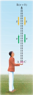
- When an object is thrown straight upwards near the surface of the earth, the velocity is zero at the maximum height that the object reaches, the acceleration is not zero.
- An object's acceleration does not determine the direction of motion of the object.
- The final velocity of an object when dropped from some height above ground is not zero. The kinematic equations do not know that the ground is there, thus the final velocity is the velocity of the object just before it actually hits the ground.
- Consider the sign of the velocity while talking about whether it is speeding up or slowing down. If the acceleration is positive and velocity is also positive then that object is speeding up in the positive direction. Moreover, if the acceleration is negative and velocity is also negative the object is speeding up in negative direction. On the contrary if the velocity and acceleration has opposite directions such as acceleration is positive and velocity is negative or vice versa the object is slowing down.
- A high magnitude of velocity does not imply anything about the acceleration. There can be a low acceleration magnitude or a high acceleration magnitude regardless of the magnitude of velocity.
- The displacement of an object does not depend on the location of your coordinate system.
Pro Tips
- Draw a physical representation of the scenario in the problem. Include initial and final velocity vectors, displacement vector, and acceleration vector.
- Place a coordinate system on the physical representation. Location of the origin does not matter, but some locations make the math easier than others (i.e. setting the origin at the initial or final location sets the initial or final position to zero).
- Always identify and write down the knowns and unknowns.
- Be very strict with labeling the kinematic variables; include subscripts indicating which object they are associated with, the coordinate, information about what stage if a multi-stage problem, and initial/final identifications. Doing this early on will help avoid the common mistake of misinterpreting the meanings of the variables when in the stage of algebraically solving the kinematic equations.
Multiple Representations
Multiple Representations is the concept that a physical phenomena can be expressed in different ways.
Physical
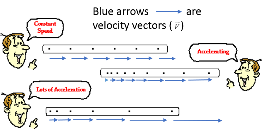
1D motion diagrams are utilized to describe the speed of an object and whether or not the object has any acceleration.
Mathematical
Watch Professor Matt Anderson explain 1D Kinematics equations using the mathematical representation.
Kinematics equations in 1D
Graphical
The Physics Classroom introduces the relationship between kinematics equations and their graphical representation. In addition, for a more in-depth discussion please refer to the graphical analysis section.
![]()
Descriptive
Example: An object undergoing parabolic (y = x^2) positional motion will have a linear (y= mx+b) velocity curve, and an acceleration curve of a constant value (y = constant).
(this example illustrates all of the most complex cases of motion studied in Kinematics, which requires constant acceleration)
Experimental
For example, a person throws a ball upward into the air with an initial velocity of $15.0 \frac{m}{s}$ . You can calculate how high it goes and how long the ball is in the air before it comes back to your hand. Ignore air resistance.