Similar to the previous section, 1D kinematics, this section quantifies the movement of objects. This time it will take into account movement in more than one dimension, for example a car driving in a parking lot or an astronaut in outer space.
Take a look at this introduction to 2D kinematics
Pre-lecture Study Resources
Read the BoxSand Introduction and watch the pre-lecture videos before doing the pre-lecture homework or attending class. If you have time, or would like more preparation, please read the OpenStax textbook and/or try the fundamental examples provided below.
BoxSand Introduction
2-D Kinematics| 2-D Kinematics
Motion obviously is not always along a straight line and two or three dimensional analysis is required. Here we will focus on two dimensions since including the third dimension add difficulties that are not necessary to illuminate the essence of the concept. The position of an object can be defined by it's position vector,
$\overrightarrow{r}=\langle x, y \rangle$
where x and y are the coordinates of the object relative to the origin. Similarly you can define the velocity and acceleration as vectors.
$\overrightarrow{v}=\langle v_x, v_y \rangle$
$\overrightarrow{a}=\langle a_x, a_y \rangle$
The vector nature of position, velocity and acceleration, allows us to break problem down to each separate component. This means you can have a set of constant acceleration kinematic equations for just the x-component,
$x_f = x_i+v_{i_x} \Delta t + \frac{1}{2} a_x \Delta t ^2$
$v_{f_x} = v_{i_x} + a_x \Delta t$
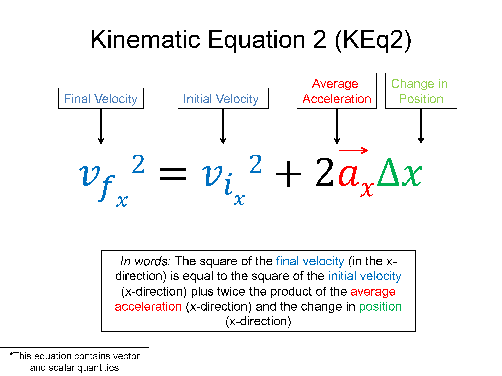
$v_{f_x}^2 =v_{i_x}^2+2a_x \Delta x$
and also a set for the y-component.
$y_f = y_i+v_{i_y} \Delta t + \frac{1}{2} a_y \Delta t ^2$
$v_{f_y} = v_{i_y} + a_y \Delta t$
$v_{f_y}^2 =v_{i_y}^2+2a_y \Delta y$
This ability to decouple the motion along one direction from another direction, perpendicular to the first, helps a great deal in analyzing motion. The feature that it brings along though, is that now you have doubled the number of kinematic variables and possible equations. Organization is key and setting up a table of known and unknown variables, for the x and y directions separately, will help with all this information.
Note that the kinematic equations can also be written in vector notation, for example,
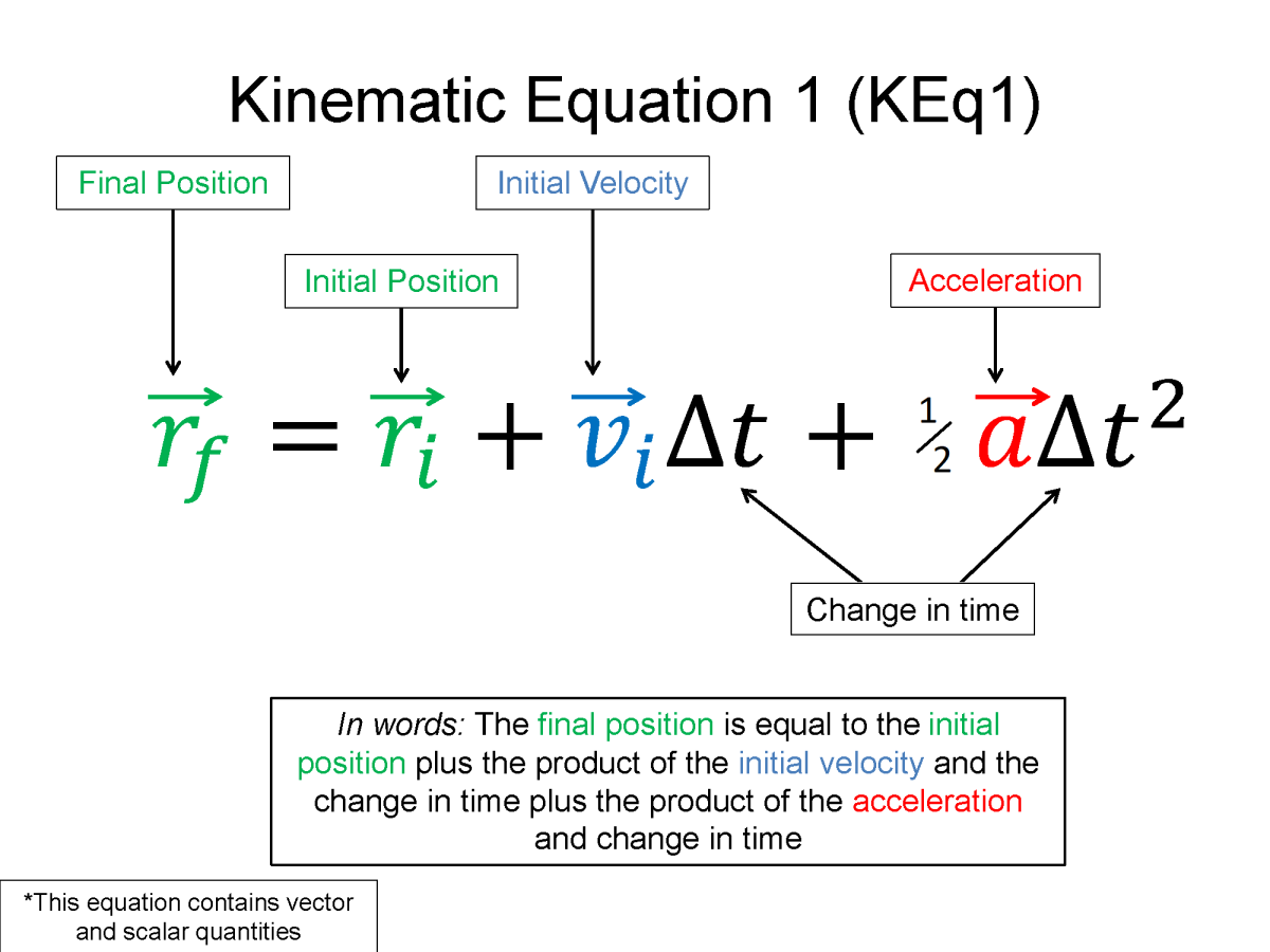
$\overrightarrow{r}_f = \overrightarrow{r}_i+\overrightarrow{v}_i \Delta t + \frac{1}{2} \overrightarrow{a} \Delta t ^2$
which implies more than one equation, one for each component, x, y, and z. When ever you see a vector symbol on anything, think of that thing being more than one thing.
The Excel File below can be used to study motion in 2 dimensions.
Click Here for 2-D Motion Excel File
Key Equations and Infographics

BoxSand Videos
Required Videos
Suggested Supplemental Videos
Exam Advice from KC
OpenStax Reading
Section 3.1 Introduces kinematics in 2-D
![]()
Section 3.2 covers vector addition and subtraction methods, which may be review at this point.
![]()
Section 3.3 expands on vector addtion and subtraction but also may be review at this point.
![]()
Fundamental examples
1. Superman initially starts from rest on level ground, then accelerates with rate of $\langle -42 , 64 \rangle \, m/s^2$.
a. If Superman is measured to be $288 \, m$ above his initial location, how long was he in flight?
b. What is Superman's displacement after the time found form part a?
c. Sketch a graph of Superman's x position as a function of time.
d. Sketch a graph of Superman's y position as a function of time.
e. Sketch the trajectory of Superman.
2. A spaceship is traveling due east with a speed of $20 \, m/s$. The spaceship's thrusters suddenly turn on and provide a constant acceleration in the southwest direction for $4$ seconds. The crew was able to determine only the south component of acceleration, which was $3 \, m/s^2$, and that they had an east component of displacement that was $40$ meters. What was the magnitude and direction of the acceleration?
CLICK HERE for solutions.
Short foundation building questions, often used as clicker questions, can be found in the clicker questions repository for this subject.
![]()
Post-Lecture Study Resources
Use the supplemental resources below to support your post-lecture study.
Practice Problems
BoxSand's Quantitative Practice Problems
BoxSand's Multiple Select Problems
Recommended example practice problems
Set 1: Problems 1 and 2, 3 if you're feeling adventurous
For additional practice problems and worked examples, go here.
For additional practice problems and worked examples, visit the link below. If you've found example problems that you've used please help us out and submit them to the student contributed content section.
![]()
Additional Boxsand Study Resources
Additional BoxSand Study Resources
Learning Objectives
Summary
Students will extend what they learned in 1-D kinematics into motion in 2-D and understand the features of perpendicular components. Students will also learn about the features of projectile motion.
Atomistic Goals
Students will be able to...
- Identify that the motion occurs in more than 1-dimension and requires a 2-D analysis.
- Define a coordinate system that simplifies the complexity of the vector analysis.
- Construct a physical representation the involves multiple dimensions and show a representation of the vector components.
- Demonstrate the ability find the Cartesian components of a vector in the mathematical representation.
- Identify known and unknown quantities for each object, stage, and dimension.
- Solve for a desired unknown in the mathematical representation using a set of kinematic equations for each dimension. Use the problem solving skills developed in 1-D kinematics
- Identify which quantities are the same when comparing two different dimensions, objects, or stages, e.g. elapsed time is the same for both x and y motion.
- Define projectile motion.
- Show that in projectile motion the acceleration has a magnitude of g = 9.8 m/s2 and points downward.
- Show that in projectile motion time of flight is determined in an analysis of the vertical motion.
- Show that in projectile motion the horizontal motion can be the same between two cases even when the vertical is not.
- Show that in projectile motion range depends on both the horizontal speed and the time of flight, thus dependent on both the vertical and horizontal analysis.
- Show that in projectile motion the range is the same for complementary angles.
- Show that in projectile motion any system can be analyzed using only the fundamental kinematics equations for constant acceleration, e.g. you do not need specially derived equations like the range equation.
- Apply limiting cases sense-making procedures to check their solutions.
YouTube Videos
Simulations
This PhET simulation allows you to drag a ball around in 2-D while visualizing the velocity and acceleration vectors.
![]()
For additional simulations on this subject, visit the simulations repository.
![]()
Demos
History
Oh no, we haven't been able to write up a history overview for this topic. If you'd like to contribute, contact the director of BoxSand, KC Walsh (walshke@oregonstate.edu).
Physics Fun
Oh no, we haven't been able to post any fun stuff for this topic yet. If you have any fun physics videos or webpages for this topic, send them to the director of BoxSand, KC Walsh (walshke@oregonstate.edu).
Other Resources
This link provides a discussion about a simple case of a falling object in a 2D system:
![]()
This link provides a introduction to simple projectile motion in a 2D system:
![]()
Resource Repository
This link will take you to the repository of other content on this topic.
![]()
Problem Solving Guide
Use the Tips and Tricks below to support your post-lecture study.
Assumptions
- Kinematics requires the assumption that acceleration is constant, if that isn't true, none of our equations or analysis techniques are necessecarily true for the motion anymore. This is often glossed over, however, as we move onto different types of analysis in the future and have multiple ways to solve problems (like say, on your final exam), the thing to remember about when you can or can't use kinematics is that the acceleration MUST be constant throughout the entire motion if you wish to analyze it with kinematics.
- Motion in one direction, x or y for example, does not imply or interfere with the motion in the other direction, provided those direction are perpindicular to each other (which all the coordinate systems we'll use in this class are).
- The ONLY thing common between the perpindicular directions in 2D kinematics is time, so often that can be used to bridge the gap in information between one direction and another.
Checklist
1. Read and re-read the whole problem carefully.
2. Visualize the scenario. Mentally try to understand what the object is doing.
a. Motion diagrams are a great tool here for visual cues as to what the motion of an object looks like.
3. Draw a physical representation of the scenario; include initial and final velocity vectors, acceleration vectors, position vectors, and displacement vectors.
4. Define a coordinate system; place the origin on the physical representation where you want the zero location of the x and y components of position.
5. Identify and write down the knowns and unknowns.
6. Identify and write down any connecting pieces of information.
7. Determine which kinematic equation(s) will provide you with the proper ratio of equations to number of unknowns; you need at least the same number of unique equations as unknowns to be able to solve for an unknown.
8. Carry out the algebraic process of solving the equation(s).
a. If simple, desired unknown can be directly solved for.
b. May have to solve for intermediate unknown to solve for desired known.
c. May have to solve multiple equations and multiple unknowns.
d. May have to refer to the geometry to create another equation.
e. If multiple objects or constant acceleration stages or dimensions, there is a set of kinematic equations - something will connect them.
9. Evaluate your answer makes sense, are the units and dimensions correct and the results are within reason.
Misconceptions & Mistakes
- An object's acceleration does not determine the direction of motion of the object.
- When an object is thrown upwards at an angle near the surface of the earth, the y-component of velocity is zero at the maximum height that the object reaches, the acceleration is not zero.
- Remember that the velocity in one direction does not imply velocity in another.
- The displacement of an object does not depend on the location of your coordinate system.
- The final velocity of an object when dropped from some height above ground is not zero. The kinematic equations do not know that the ground is there, thus the final velocity is the velocity of the object just before it actually hits the ground.
Pro Tips
- Draw a physical representation of the scenario in the problem. Include initial and final velocity vectors, displacement vector, and acceleration vector.
- Place a coordinate system on the physical representation. Location of the origin does not matter, but some locations make the math easier than others (i.e. setting the origin at the initial or final location sets the initial or final position to zero).
- Always identify and write down the knowns and unknowns.
- Be very strict with labeling the kinematic variables; include subscripts indicating which object they are associated with, the coordinate, information about what stage if a multi-stage problem, and initial/final identifications. Doing this early on will help avoid the common mistake of misinterpreting the meanings of the variables when in the stage of algebraically solving the kinematic equations.
- Remember in 2D kinematics problems is that the two dimensions are entirely independent of each other. Treat them separately, come up with the knowns and unknowns for all variables in each direction.
- The only connection between the two dimensions is time, often it will serve as a means to connect the two seperate directions and sets of knowns and unknowns.
- Keep track of your angles and break all forces in various directions into their components in your chosen coordinate system.
Multiple Representations
Multiple Representations is the concept that a physical phenomena can be expressed in different ways.
Physical
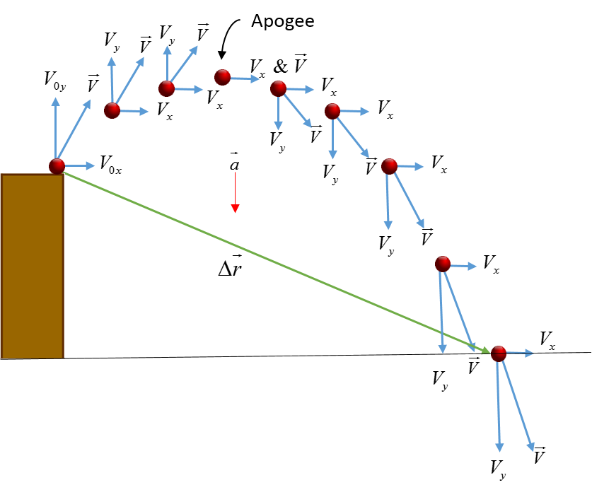
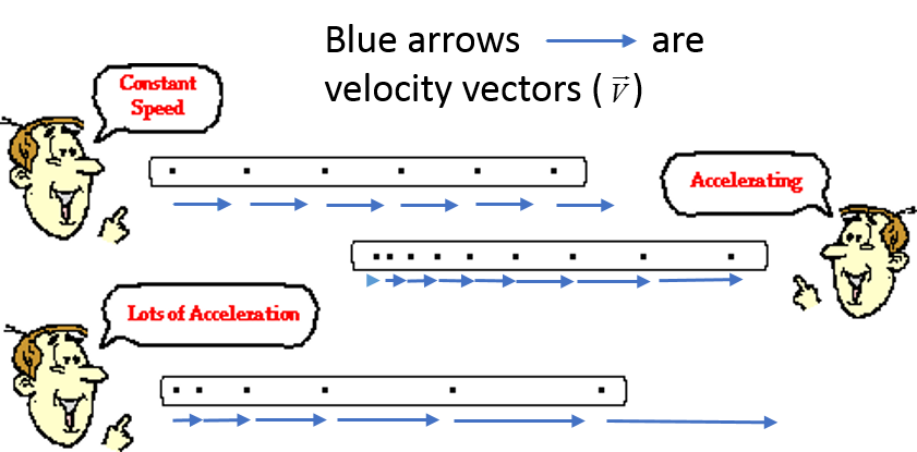
Kinematics problems are often analyzed with physical descriptions. Below we have an object launched from a ledge with initial horizontal and vertical velocity components. The vectors indicate the relative magnitudes of the horizontal and vertical velocity components at different stages of the objects motion.
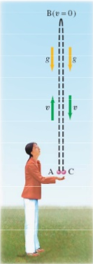
In addition, simple 1D motion diagrams are utilized to describe the speed of an object and whether or not the object has any acceleration.
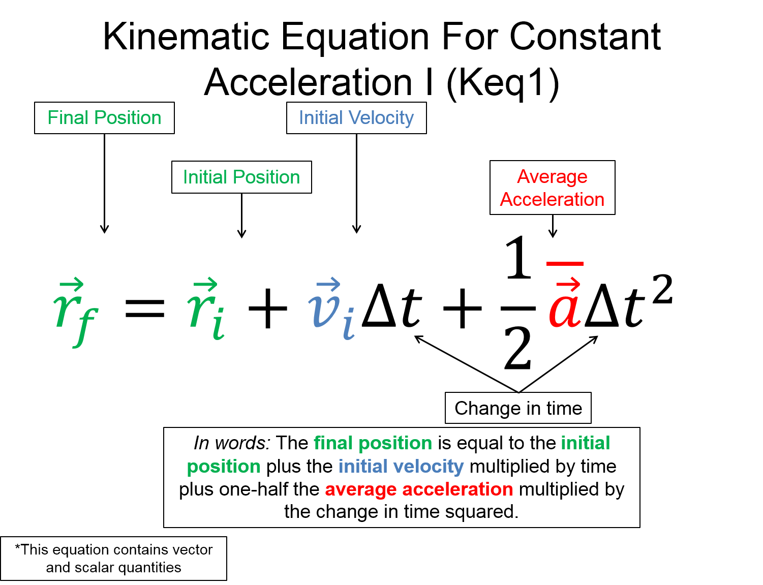
Mathematical
Main kinematics equations. Notice that we use $ r $ to represent the vector position. In the videos below, Professor Matt Anderson uses $ x $ and $ y $ to denote position in a given coordinate direction.
$ \vec{r}_{f} = \vec{r}_{i}+\vec{v}_{i} \Delta t + \frac{1}{2} \vec{a} \Delta t^{2} $
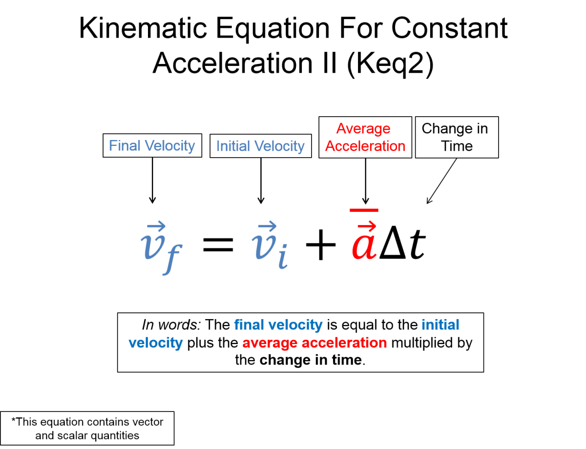
$ \vec{v}_{f} = \vec{v}_{i} + \vec{a} \Delta t $
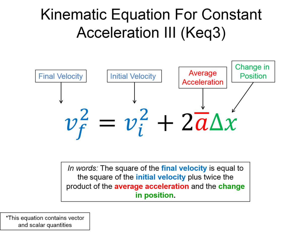
$ v_{fx}^{2} = v_{ix}^{2}+2a_{x} \Delta x $
Watch Professor Matt Anderson explain 1D and 2D Kinematics equations using the mathematical representation.
Video 1: Kinematics equations in 1D
Video 2: Kinematics equations in 2D
Graphical
the Physics Classroom introduces the relationship between kinematics equations and their graphical representation. In addition, for a more in-depth discussion please refer to the graphical analysis section.
![]()
Descriptive
The branch of mechanics concerned with the motion of objects without reference to the forces that cause the motion.
Experimental
For example, a person throws a ball upward into the air with an initial velocity of $15.0 \frac{m}{s}$. You can calculate how high it goes and how long the ball is in the air before it comes back to your hand. Ignore air resistance.