What is a Radian? This video helps you visualize the concept.
https://www.youtube.com/watch?v=Ac453CO3ysQ
Pre-lecture Study Resources
Watch the pre-lecture videos and read through the OpenStax text before doing the pre-lecture homework or attending class.
BoxSand Videos
Required Videos
Suggested Supplemental Videos
Learning Objectives
Summary
The objective is to analyze non-uniform circular motion with emphasis on angular position, velocity, and acceleration in both the mathematical and graphical representation. Special emphasis is placed on relating the rotational to the translational motion analysis.
Atomistic Goals
Students will be able to...
- Identify systems where the motion can be decomposed into translational and rotational behavior.
- Identify systems that can be analyzed with any combination of a radial, tangential, and axial velocity components.
- Define rotational motion as an object traveling in a circle.
- Show that rigid-body rotation can be analyzed using the same analysis tools as point particle circular motion.
- Differentiate between polar and Cartesian coordinate systems and identify that a polar system reduces rotational motion from a 2-D analysis in Cartesian, to a 1-D analysis in polar coordinates.
- Apply polar coordinates to analyze rotational motion.
- Demonstrate that UCM and non-UCM only have tangential velocity components.
- Identify UCM systems having only a radial component of acceleration while non-UCM have both radial and tangential acceleration components.
- Define the angular position theta.
- Convert between radians, degrees, revolutions
- Apply the equation for the average angular velocity omega.
- Apply the equation for the average acceleration alpha.
- Use the sign convention to identify whether the angular displacement and thus angular velocity are positive or negative.
- Use the rules learned in translational motion about whether something is speeding or slowing, to determine if the angular acceleration is positive or negative.
- Identify and apply the similarities of a graphical analysis for rotational kinematics with that from translational kinematics.
- Recognize the form-like invariance between the rotational and translational kinematic equations for constant acceleration and apply them to rotational motion using the methods learned in translational kinematics.
- Recognize the relationship between period and frequency and be able to calculate one from the other.
- Differentiate between frequency and angular velocity and be able to calculate one from another.
- Drop the units of radians when appropriate because they are a dimensionless parameter.
- Apply the relationship between the arc length and the change in angle, via the radius.
- Apply the relationship between the tangential component of velocity and angular velocity, via the radius.
- Apply the relationship between the tangential component of acceleration and angular acceleration, via the radius.
- Apply the relationship between the radial component of acceleration and the square of the tangential component of velocity, via the radius.
- Combine the definition of the tangential velocity and the angular velocity to show the relationship between the radial component of the acceleration and the angular velocity, via the radius.
- Identify locations in a system that have the same angular velocity but different translational speed.
BoxSand Introduction
Rotational Kinematics | Connecting Rotational and Translational Kinematics
Going Between Angular and Linear: Now that we see what the rotational kinematic variables are, and how the equations for constant acceleration allows you to use them to find instantaneous values, it's important to see how they can also be used to find their linear counterparts. Some problems may state what the initial and final angular velocities are, and the change in angle during that motion, then ask for the time. In that case you would not have to use any of the linear quantities to solve the problem. Although it then asks what the linear speed was at the end of the motion, you'd have to use the following relationships below.
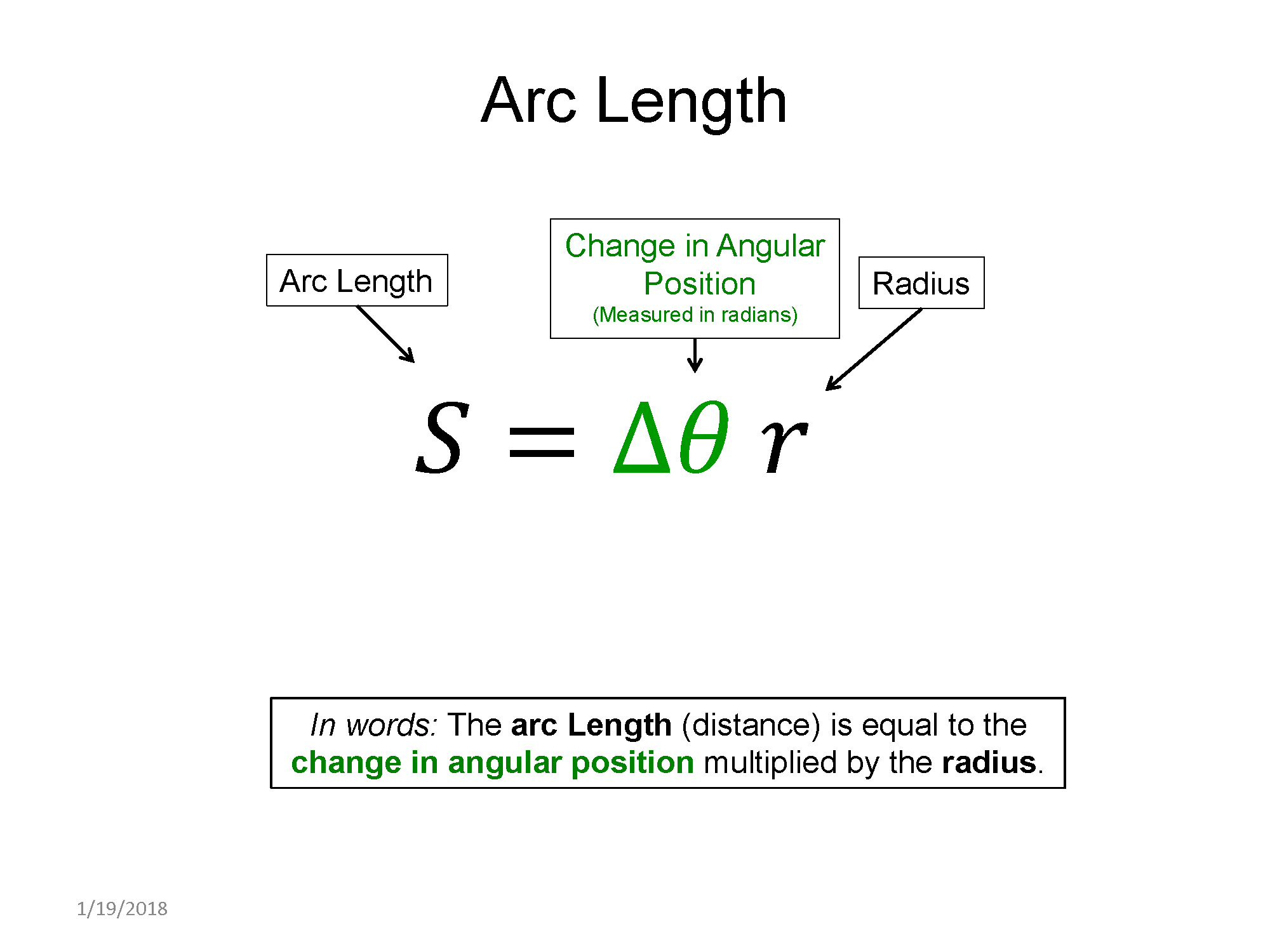
Change in angular position ==> Distance traveled: $s=\Delta \theta r$
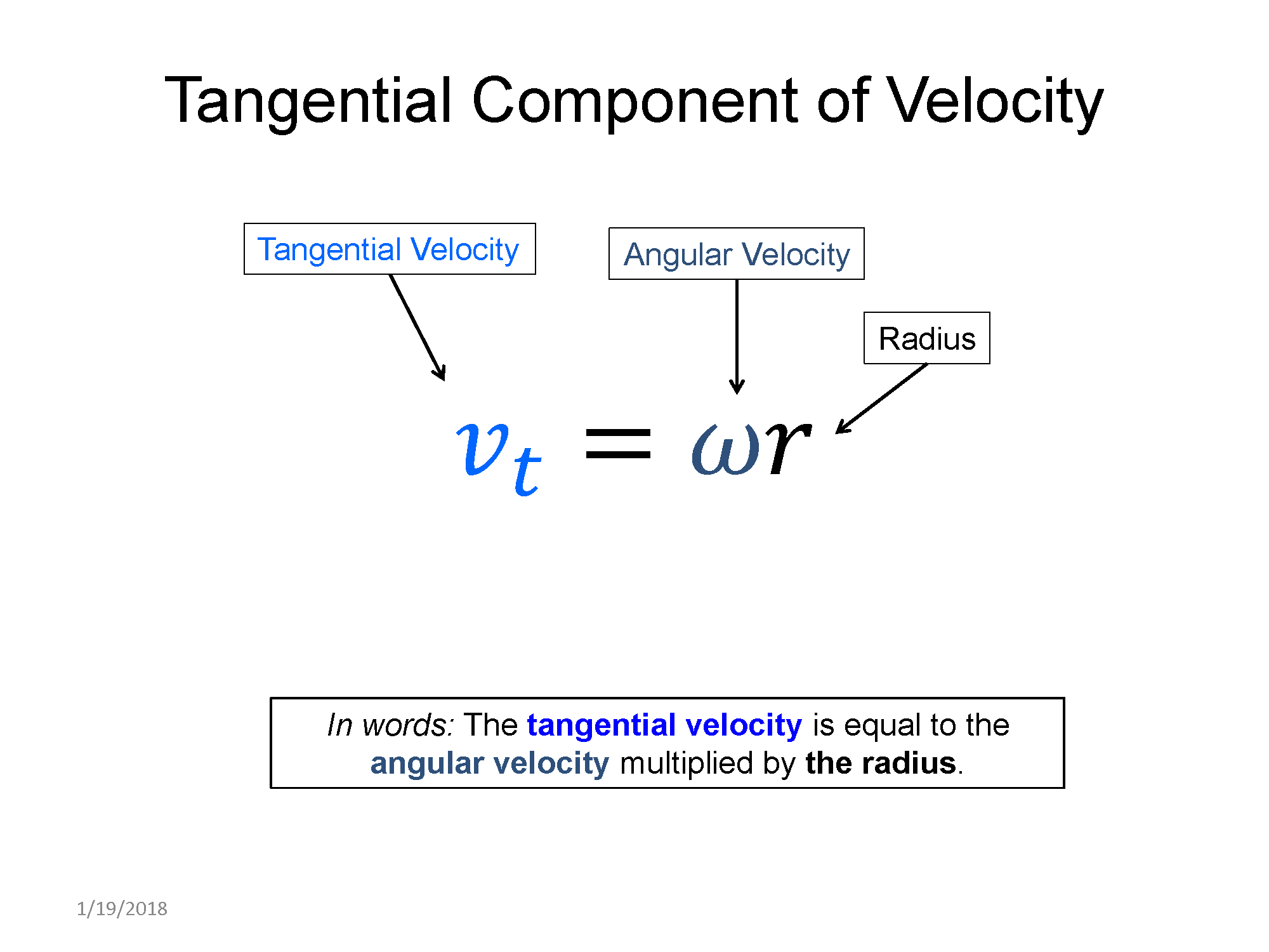
Angular velocity ==> speed: $|\overrightarrow{v}| = v_t = \omega r$
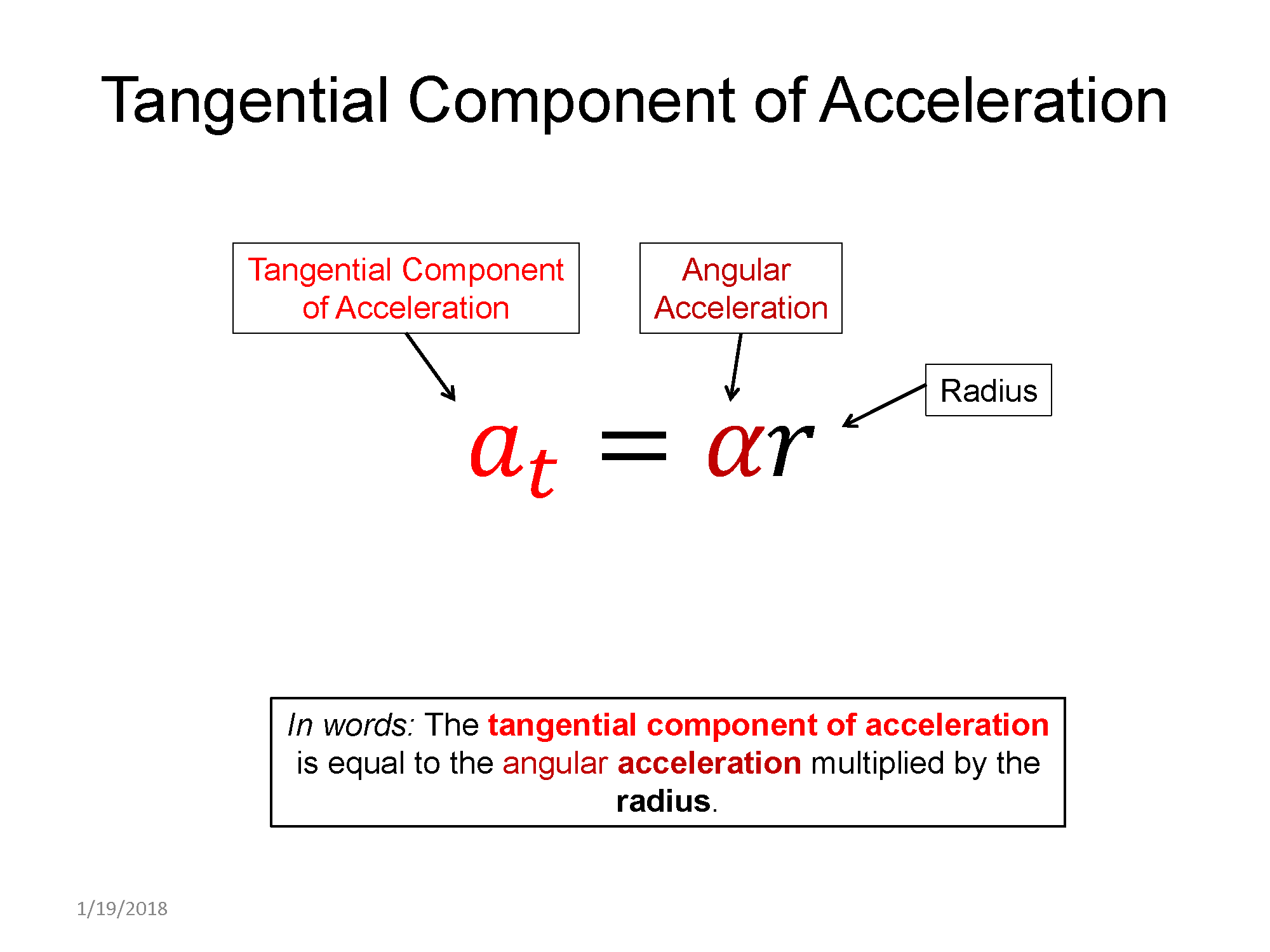
Angular acceleration ==> Tangential component of linear acceleration: $a_t = \alpha r$
The linear coordinate system we use in this case is one with a radial inward direction ($\widehat{r}$), a CCW tangential direction ($\widehat{t}$), and a direction perpendicular to those two ($\widehat{z}$). This means that since the object is always traveling tangent to the circle, the linear velocity has zero radial or z components - the speed of the object is equal to the tangent component of its linear velocity.
$\overrightarrow{v}=\langle v_r, v_t, v_z \rangle = \langle 0, \omega r, 0 \rangle$
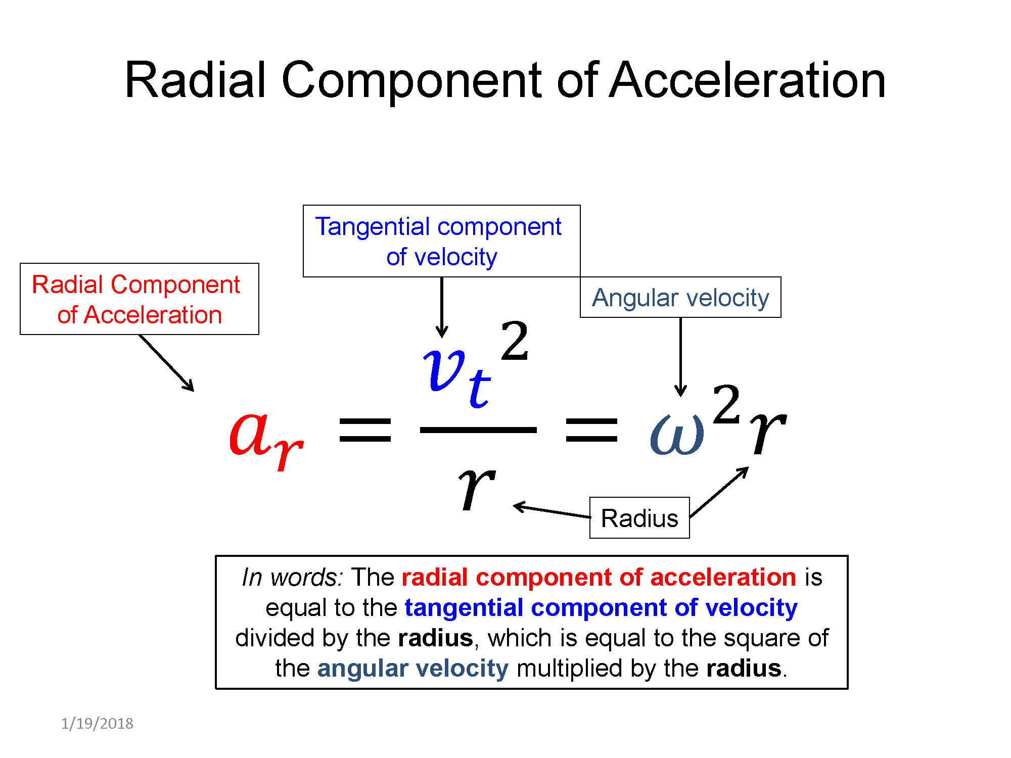
For the angular acceleration, using the same $\widehat{r}$,$\widehat{t}$, and $\widehat{z}$, coordinate system, the object has zero z component to its acceleration. If you recall though it does have a radial component equal to the square of its speed divided by the radius of the circle its traversing ($a_r = \frac{v^2}{r}$). The full linear acceleration is thus:
$\overrightarrow{a}=\langle a_r, a_t, a_z \rangle = \langle \frac{v^2}{r}, \alpha r, 0 \rangle$
Key Equations and Infographics

Now, take a look at the pre-lecture reading and videos below.
OpenStax Reading
(Same as the previous lecture)
OpenStax Section 10.1 | Angular Acceleration
![]()
OpenStax Section 10.2 | Kinematics of Rotational Motion
![]()
Additional Study Resources
Use the supplemental resources below to support your post-lecture study.
YouTube Videos
Crash Course Physics provides a great introduction to rotational motion.
https://www.youtube.com/embed/fmXFWi-WfyU
Flipping Physics provides a great review of rotational kinematics
https://www.youtube.com/watch?v=DoZ6Sjy4LaU
Here Khan Academy explains the smiliarties between the translational and rotational kinematics equations
https://www.youtube.com/watch?v=TBlDBaUGqNc
Non-uniform rotational mechanics
https://www.youtube.com/watch?v=p21oe2m0H3w
Here Khan Academy explains the similarities between the translational and rotational kinematics equations
Simulations
This PhET simulation has a rich interface to change a variety of parameters of a ladybug undergoing nUCM. See if you can set it to rotate one direction initially but then slow down and eventually rotate the other direction. Note what physical parameters, e.g. relative sign of omega and alpha, are required for this type of motion.
![]()
For additional simulations on this subject, visit the simulations repository.
![]()
Demos
For additional demos involving this subject, visit the demo repository
![]()
History
Oh no, we haven't been able to write up a history overview for this topic. If you'd like to contribute, contact the director of BoxSand, KC Walsh (walshke@oregonstate.edu).
Physics Fun
Other Resources
Hyperphysics covers basic rotational quantities, angular velocity, description of rotation, and rotational kinematics equations.
![]()
This website provides another overview of rotational kinematics with example problems to introduce variables.
![]()
The Physics Classroom covers the subject of Centripetal Acceleration(caused by the centripetal force of course)
![]()
Resource Repository
This link will take you to the repository of other content related resources.
![]()
Problem Solving Guide
Use the Tips and Tricks below to support your post-lecture study.
Assumptions
- The assumptions made for rotational kinematics are very similar to the assumptions for linear kinematics, we just use rotational quantities and verbage instead of our regular kinematics verbage. The core assumption that made kinematics viable was that acceleration is equal to a constant (a number), for roatational kinematics, angular acceleration ($\alpha$) must be constant.
- Just like regular kinematics, there are 5 variables we care about: Angular acceleration ($\alpha$), intial and final angular velocity($\omega_i, \omega_f$), change in angular position ($\Delta \theta$), and change in time ($\Delta t$). All the equations have 4 variables in them, meaning you need to know 3 to start using them. The best strategy for solving problem after getting the grasp of what is physically happening (like with a picture!) is to take inventory of what variables you're given, with the goal of getting 3, then move on to using the equations!
- Like before, there are some bits of verbage that should signal speicfic assumptions in problems. If angular velocity is held constant, that means $\alpha=0$. Likewise if a problem says a system is in rotational equalibrium (static OR dynamic, both have $\alpha=0$, for static rotational equalibrium $\omega=0$ as well).
Checklist
All of the lessons learned while practicing linear kinematic problems are relevant when solving rotational kinematic problems.
- Visualize the motion of the object(s) in question.
- Identify your system - this can be aided by drawing a dotted line around your system.
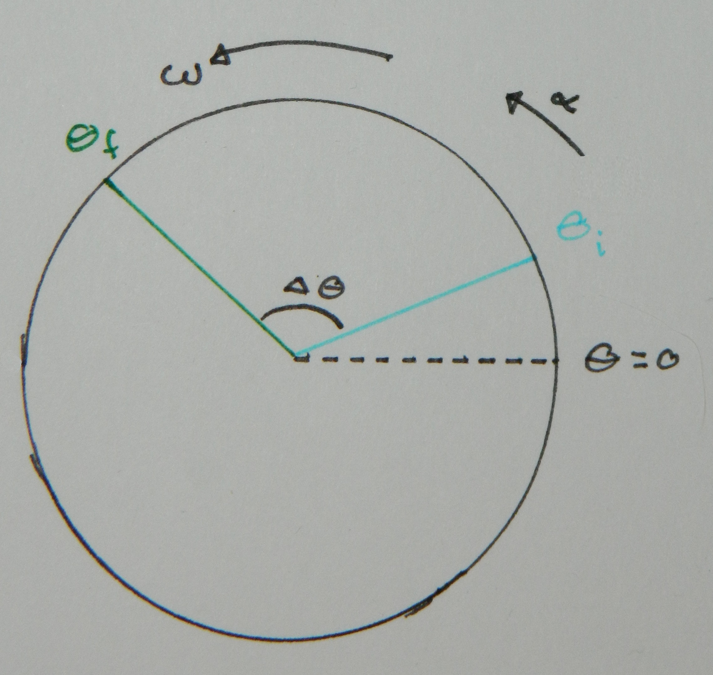
- Draw a physical representation. A physical representation is not just a pretty picture but rather a simple figure that includes a representation of important physical quantities such as angular velocity. The diagram should include a representation of initial and final angular velocity, angular acceleration, change in angle, and (sometimes) time. An example for an object slowing down is below.
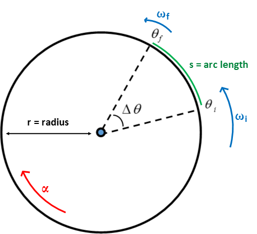
- Identify known and unknown quantities. That means for each stage/object in the system there are five kinematic quantities ($\Delta \theta, \omega_i, \omega_f, \alpha, t$ to put in a known or unknown category. Follow the convention of CCW being positive for the sign of each quantity. For example in the above figure, the initial and final angular velocities are in the CCW direction and thus would be positive. The angular acceleration though, since the object is slowing down, points in the opposite direction as the velocity and thus is CW and would be a negative number.
- Use the kinematic equations of constant acceleration to solve for the unknown quantities.
-
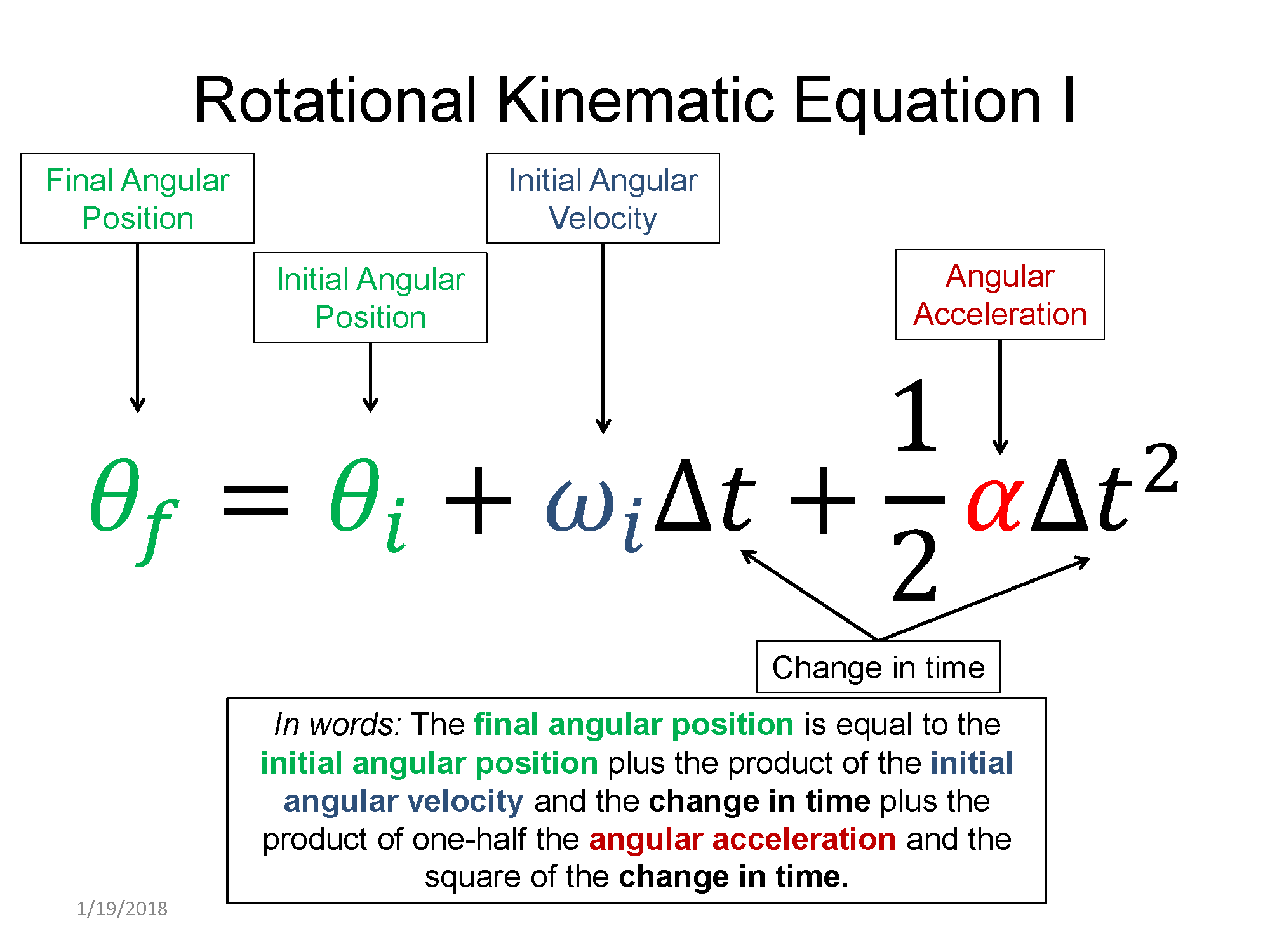
- $\Delta \theta = \omega_i \Delta t + \frac{1}{2} \alpha \Delta t^2$
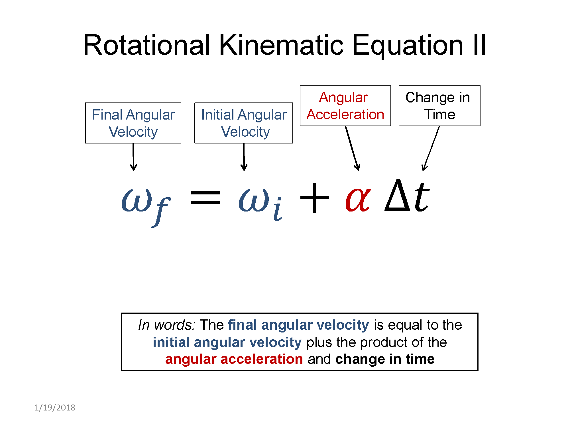
- $\omega_f = \omega_i + \alpha \Delta t$
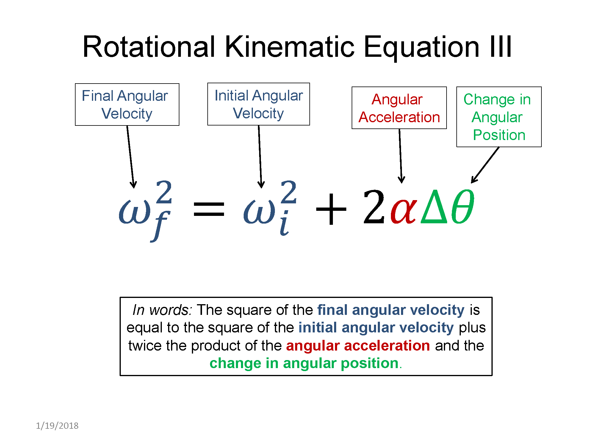
- $\omega_f^2 = \omega_i^2 + 2 \alpha \Delta \theta$
-
This may require solving simultaneous equations. One way to approach this step is to find the same number of equations as number of unknowns. It then mathematically can be solved.
- Lastly, and especially if you get stuck in part 5, remember there are connections between the angular and linear kinematic variables. This may be used to give you a new equation with no new unknowns or to simply change your answer from an angular to linear value. An example might be after finding the object subtended 2 Rads, you convert that to the distance it traveled in meters. Use the connections between the linear and angular variables below.
Change in angular position ==> Distance traveled: $s=\Delta \theta r$
Angular velocity ==> speed: $|\overrightarrow{v}| = v_t = \omega r$
Angular acceleration ==> Tangential component of linear acceleration: $a_t = \alpha r$
$\overrightarrow{v}=\langle v_r, v_t, v_z \rangle = \langle 0, \omega r, 0 \rangle$
$\overrightarrow{a}=\langle a_r, a_t, a_z \rangle = \langle \frac{v^2}{r}, \alpha r, 0 \rangle$
Misconceptions & Mistakes
-
Differentiate between radial acceleration and tangential acceleration. The radial acceleration, $a_r$ is along the radius. If the speed is not constant, then there is also a tangential acceleration, $a_t$. The tangential acceleration is, indeed, tangent to the path of the particle's motion.
-
Convention defines positive as counter-clockwise (CCW), and negative as clockwise (CW) motion.
-
Consider the sign of the angular velocity while talking about whether it is speeding up or slowing down. If the acceleration is positive and velocity is also positive then that object is speeding up in the positive direction. Moreover, if the acceleration is negative and velocity is also negative the object is speeding up in negative direction. On the contrary if the velocity and acceleration has opposite directions such as acceleration is positive and velocity is negative or vice versa the object is slowing down.
- A high magnitude of velocity does not imply anything about the acceleration. There can be a low acceleration magnitude or a high acceleration magnitude regardless of the magnitude of velocity.
Pro Tips
- A lot of the reasoning you use in rotational kinematics is the same as the reasoning you used in linear kinematics, just now things are rotating. Re-read some notes (or KC's lecture vids) from last quarter as a refresher.
- Check the units as you go, pay special attention to degrees vs radians.
- Always identify and write down the knowns and unknowns.
- The circumference of the circle created by the motion can be used for the angular position of the object.
- Be very strict with labeling the kinematic variables; include subscripts indicating which object they are associated with, the coordinate, information about what stage if a multi-stage problem, and initial/final identifications. Doing this early on will help avoid the common mistake of misinterpreting the meanings of the variables when in the stage of algebrically solving the kinematic equations.
Multiple Representations
Multiple Representations is the concept that a physical phenomena can be expressed in different ways.
Physical
$\theta$ is the angular position, $\omega$ is the angular velocity, $\alpha$ is the angular acceleration.
Mathematical
$\Delta \theta = \omega_i \Delta t + \frac{1}{2} \alpha \Delta t^2$
$\omega_f = \omega_i + \alpha \Delta t$
$\omega_f ^2 = \omega_i^2 + 2\alpha \Delta \theta$
The relations between angular and linear,
$S = \Delta \theta r $, $v_{\text{tangential}} = \omega r$, $a_{\text{tangential}} = \alpha r$
Angular frequency ($\omega$), Angular acceleration ($\alpha$)
Graphical
Below is the plot of the angular position ($\theta$) as a function of time for some object increasing its speed will traveling in a circle.
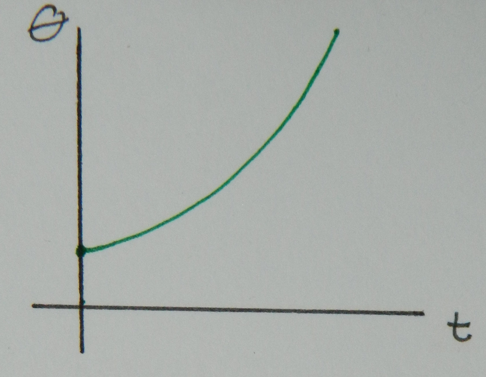
The slope of the position plot, this time measured as an angle, with respect to time is equal to the angular velocity ($\omega$). This is no different than in linear motion where velocity is the slope of position. Since the slope of the angular position as a function of time is increasing, that behavior is displayed in in the angular velocity as a function of time below.
$\omega = \frac{\Delta \theta}{\Delta t}$
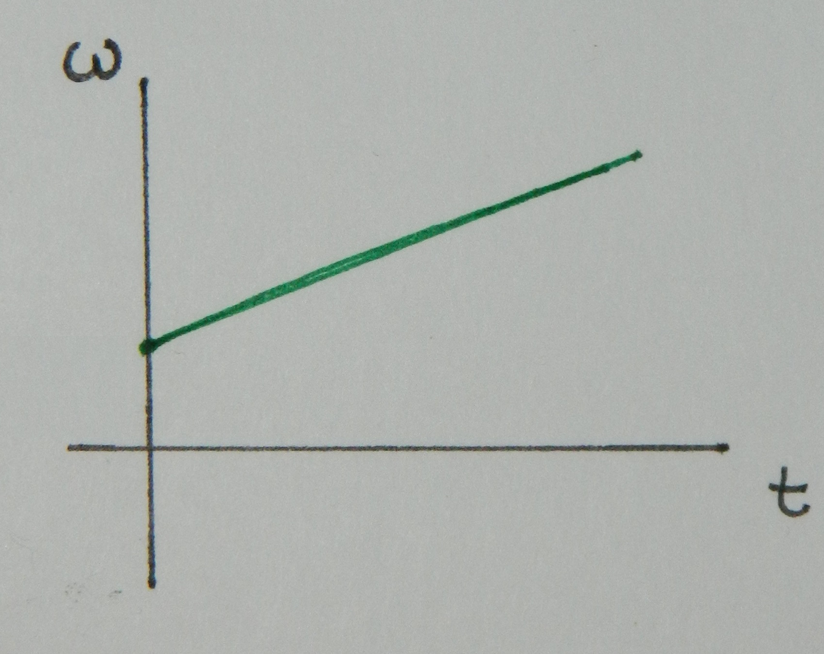
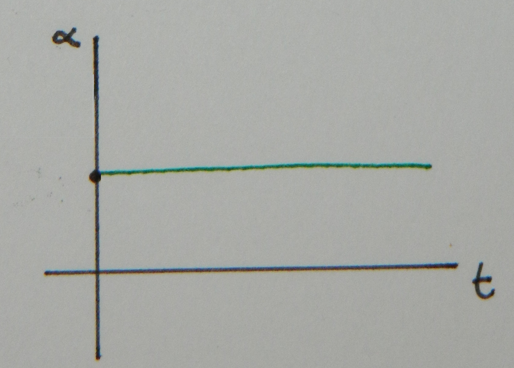
The angular acceleration ($\alpha$) is the slope of the angular velocity. Since the slope of the above plot is constant, the value of the angular acceleration is a constant, as shown below.
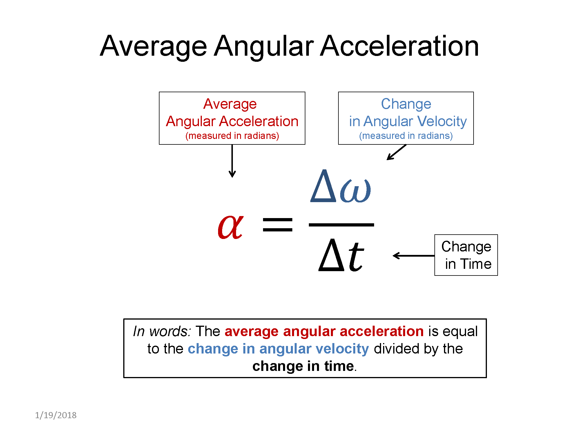
$\alpha = \frac{\Delta \omega}{\Delta t}$
This is analogous to the linear position, velocity, and acceleration graphs, which means that to go the other way, like from acceleration to velocity, you'd use the area under the plot.
Descriptive
At $t_i$ a disk is spinning with an angular velocity of $\omega_i$, with an angular acceleration of $\alpha$. After t seconds the disk has and angular velocity of $\omega_f$, and has experienced a change in angular position $\Delta \theta = \omega_i \Delta t + \frac{1}{2} \alpha \Delta t^2$.
Experimental
You can setup an experiment to study the phenomena of constant angular acceleration. An example is demonstrated below.
Practice
Use the practice problem sets below to strengthen your knowledge of this topic.
Fundamental examples
1. A Beckman type 75 Ti centrifuge rotor is rated for a maximum frequency of $75,000$ RPM. At this maximum frequency, how much time will it take for the rotor to complete $10,000$ revolutions?
2. Pretend that a Beckman ultracentrifuge has a constant angular acceleration of $20 \, rad/s^2$.
(a) How long will it take for a rotor, starting from rest, to reach a frequency of $30,000$ RPM?
(b) How many revolutions did the rotor complete in this amount of time?
3. The rotational motion of a wheel is described by the graph below.
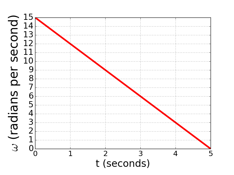
(a) What is the angular acceleration of this wheel?
(b) Through how many radians did the wheel travel through from 0 to 5 seconds?
CLICK HERE for solutions.
Short foundation building questions, often used as clicker questions, can be found in the clicker questions repository for this subject.
![]()
Practice Problems
Recommended example practice problems
Set 1: UofW-Green Bay: Accelerating Merry-Go-Round, Website Link
Set 2: PSTCC: A section self test and example problems on the bottom half of the page, Website Link
Set 3: Rotational mechanics of a bullet and rifle, Website Link
Coffin's practice problems
For additional practice problems and worked examples, visit the link below. If you've found example problems that you've used please help us out and submit them to the student contributed content section.