Required Videos

Suggested Supplemental Videos

Summary

Summary

Atomistic Goals

Students will be able to...

1.  

Resistive Circuits | Micro-model of Charge flow, Resistance, Ohm's Law, Power

 

Imagine a neutral conductor, for example a thin metal rod, that is not in the presence of any external electric field. Relying on our microscopic model of matter, we can describe this metal rod as a mix of free electrons uniformly distributed throughout the volume of the rod, and tightly bound electrons in the vicinity of their corresponding positive ion cores that make up the lattice. Now imagine turning on an external electric field, for example a uniform electric field parallel to rod. Can you predict what will happen to the metal rod? Hopefully you were thinking along the lines of, "polarization". The instant the conductor finds itself inside this electric field, the free electrons feel a force due to their interaction with the electric field. This force causes the free electrons to migrate from their current location, anywhere within the rod, to the end of the rod. The migration of these electrons cannot last forever and eventually an electrostatic condition is established where one end of the rod is now more negatively charged than the other end and no more free electrons are moving towards the negative end. It turns out that the time it takes the rod to reach this electrostatic condition and become polarized happens extremely quick, on the order of microseconds or even faster. Nevertheless, we say that there is an electric current during the short time when the free electrons are moving towards the end. The electric current, or current for short, ceases to exist when the electrostatic condition is reached, after all no more free electrons would moving towards the end. In the upcoming lectures we will look at ways to establish a current that last quite a long time, seconds, minutes, hours, and even days or years. We will then study some of the applications of current, but for now this lecture will focus on developing a classical microscopic model of current. I emphasize "classical" because our microscopic model is far different than the modern quantum model. Even though a more robust model is found by invoking principles of quantum mechanics, the classical model we will develop correctly predicts common observations of the quantities related to current. Since this is an course focused on classical physics, I will drop the classical label as it is redundant. The microscopic model of current we wish to develop will draw upon much of your previous physics concepts such as: the features of conductors, electric fields, how forces and electric fields are related, how force and acceleration are related, how acceleration and velocity are related, and dimensional analysis. While constructing this microscopic model of current, we will encounter quantities that will be useful in characterizing devices that rely on current in order to perform their function (e.g. lightbulbs, speakers, car components, etc..). We will begin our development of the microscopic model of current with an electrostatics overview.

 

Electrostatics overview

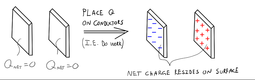
Below is a short list of some of the features of conductors. These features will be drawn upon when constructing a microscopic model of current.

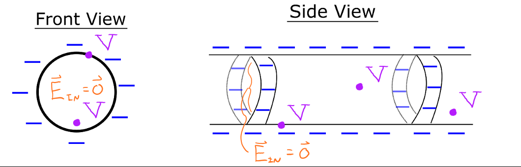
• Any net charge on a conductor resides on the surface of the conductor.
• This net charge distributes itself over the surface of the conductor such that the electric field inside the conductor is zero in electrostatic equilibrium and the electric potential (commonly referred to as voltage) is a constant within and on the surface of the conductor.
• The actual distribution of the net charge on the surface is complicated, but for highly symmetric cases the surface charge distribution is uniform (e.g. sphere or very long cylinder far away from edges).
  • Example: The net charge on a very long cylinder spreads out uniformly across the surface as shown in the diagrams below. The excess charges here are considered electrons, which are represented with a negative sign ( − ). The three dimensional nature makes it challenging to illustrate a side view. Thus, only two circular strips around the surface of the cylinder are shown for simplicity. Also note that the excess electrons distribute themselves across the surface of the cylinder in such a way that the electric field inside the cylinder is zero. The ends of the cylinder are not shown because the electrons are distributed in a complicated way around the edges which isn't important for our following discussions.
  • The purple numbers represent the electric potential at various locations. Notice that at this electrostatic equilibrium condition the electric potential is a constant. For example, V could be -10 volts at all locations.

Getting charges to accelerate

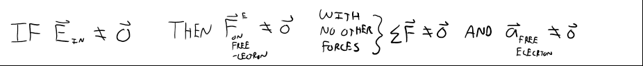
Recall that an electron will experience an electric force if it is placed an electric field; a mathematical representation of this statement is shown below:

$$\vec{F}^{E}_{on free electron} = - e \vec{E}_{in}$$

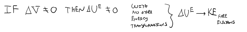
Continuing with our cylindrical conductor example, let's take a look at the free electrons contained within the cylinder. Even with a net charge on the cylinder, the free electrons do not feel an electric force because the electric field inside is zero. So how do we get the free electrons to accelerate, thereby moving (i.e. how do we create current)? One answer is to use an electric field to "push" the free electrons around the inside of the conductor. Our goal now is to determine what type of charge distribution on our cylindrical conductor will create an electric field inside the conductor, causing free electrons to accelerate thus establishing a current. We also have another equally valid way of analyzing motion of charged objects; instead of using electric fields, we can think in terms of electric potentials. Recall that an electron placed in a region of space where the electric potential is non-uniform, it will interact with the electric potential in such a way as to minimize the electric potential energy associated with the interaction of the electron and the potential field. Basically, the electron will move up in electric potential to decrease its energy. Thus another way to think about the answer to the question, how do we get charges to accelerate, is to create an electric potential gradient that the electrons can move up in. The above to paragraphs are equivalent. Remember that electric fields are connected to electric potentials, that is, if we have one we can get the other. Thus the above two paragraphs are just two different ways of looking at the same problem of getting free electrons to accelerate inside a conductor.

To summarize this section there are two equivalent ideas:

• Use electric fields to "push" free charges around inside of a conductor.

• Use an electric potential gradient to cause free charges to move inside of a conductor.

Setting up electric field inside a conductor

Now that we have determined that an electric field inside of the conductor is needed to establish a current, let's take a look at how we can accomplish this. One way would be to put a conductor inside an external electric field, like in the introduction paragraph. However, we saw that this only creates a current for a very short amount of time. Thus, we will walk through the steps of a different way to create an electric fide inside a conductor.

• Start with 2 neutral conducing wires as shown below

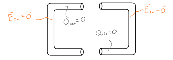
• Get 2 large neutral conducting plates. ○ Do work to place a net charge on each plate.

• Connect each plate to one of the neutral wires.

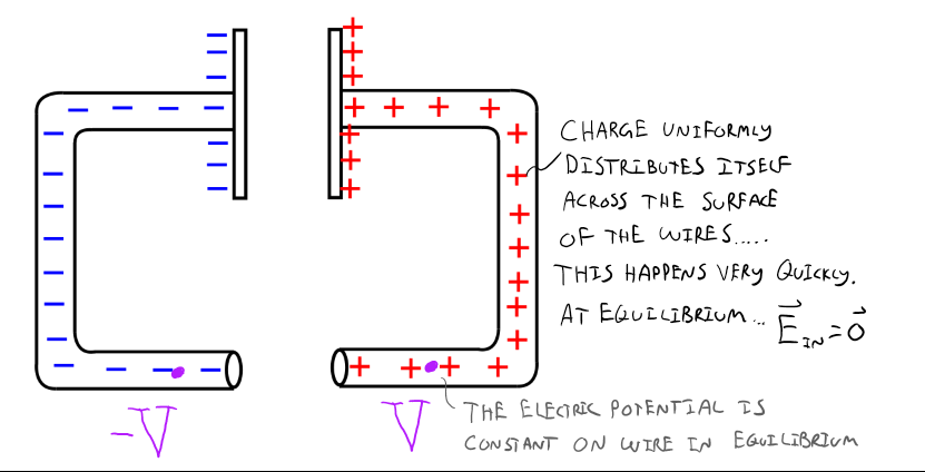
• Connect the wires at the bottom. ○
  • Once connected, the positive surface charges are attracted to the negative surface charges and they begin to "mix". A charge gradient is now present, in other words, a non-uniform surface charge distribution is now present on the surface of the wires. This process takes happens very quickly…basically instantaneous.

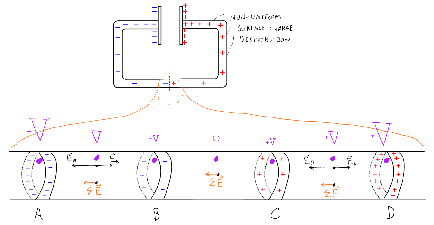
Study the above image carefully. Here we zoomed into a small segment of the wire and analyzed the electric field at three regions: between A and B, between B and C, and between C and D. Look at the region between A and B: Because there exists a surface charge gradient (i.e. the surface charge is larger in magnitude near strip A than near strip B), there is a net electric field that points to the left. The electric field analysis isn't shown for the region between B and C, but you should convince yourself that the analysis would result in a net electric field also pointing to the left. Note that the electric field vectors are not drawn to scale. The alternative way to look at the effects of the non-uniform charge distribution would be to look at the electric potential. Since the surface charge is more positive near strop D than it is at C, the electric potential is a larger positive at D than it is at C. The electric potential then continues to decrease as you move from right to left. There are a few important features we can get from this image:

• The electric field inside the wire is parallel to the wire and it will follow the direction of the wire as the wire bends.
• The non-uniform surface charge distribution creates an electric field inside the wire that the free electrons will interact with, causing them to accelerate; thus current is established so long as the non-uniform surface charge distribution exists.
  • Alternatively, the non-uniform surface charge distribution creates an electric potential gradient within the wire that the free electrons will "fall up in electric potential" in order to minimize their energy.
• Remember that the surface charges are free to move along the surface. Thus if no more charge is added to the plates, eventually the whole wire+plate system will reach electrostatic equilibrium. Thus, to maintain the current, we need to maintain the non-uniform surface charge distribution by doing work and adding more charge to the plates. Basically, we need a way to continuously separate charge to place on the plates. This is essentially what batteries do, they separate charges to maintain the non-uniform surface charge distribution of the wires they are connected to.

 

Charge carriers navigating the conductor's lattice

We now know how to establish a current, or in other words, get electrons to accelerate inside the conductor. Unfortunately, the free electrons are surrounded by a lattice of ion cores that might get in the way of the electrons as they are accelerating. Thus, in this section, we will take a closer look at the motion of the free electrons as they navigate the conductors lattice.

Recall that all objects above 0 K have random microscopic motion of its atoms. So even before we establish an electric field (or an electric potential gradient), the free electrons are actually moving around inside the conductor. A representation of their motion is shown below in the image on the left. Since there is no not force on the free electrons, they travel in straight lines until they scatter off the ion cores changing their direction. Now imagine we create that internal electric field to accelerate the electrons. With a net force on the electrons, they might travel a path as represented in the image below on the right. The free electrons will travel in parabolic trajectories until they too scatter off an ion core and change direction.

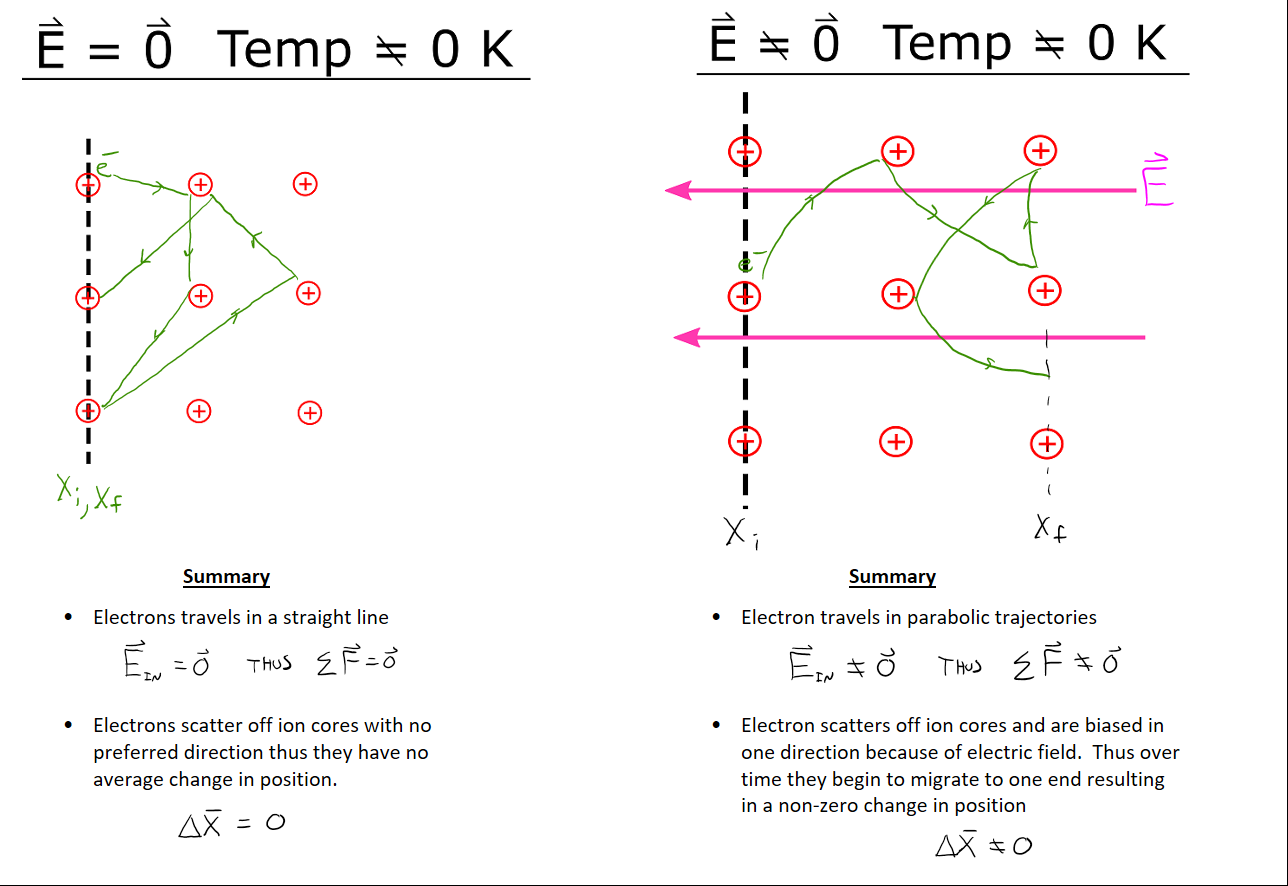
If we were able to plot the velocities of the free electrons they might look something like the graphs below. On the left is the case with no electric field inside, and the graph on the right represents the case where there is an electric field inside.

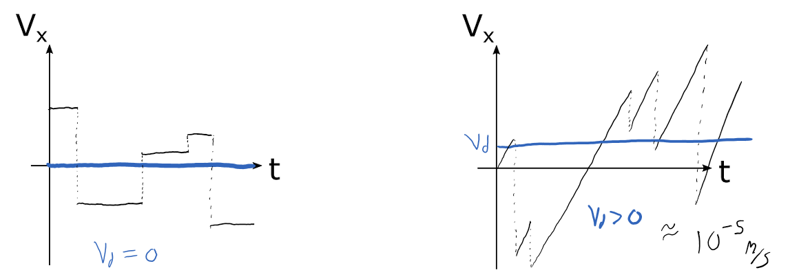
If we look at the graph on the left, notice that on average, the free electron spends just as much time with a positive velocity as it does with a negative velocity. The electrons are certainly moving in our model, but on average it looks like they are not moving since they always wind up at the same location they started. Thus we will introduce to a new term called drift speed ($v_d$) to differentiate the electron's instantaneous velocity with its overall change in position over change in time.

Now look at the graph on the right. The first thing you should notice is the linear velocities because of a constant net force. Since the free electrons always have a constant force on them due to the electric field, they will spend more time traveling in one direction (here positive) than the other direction (here negative). If we took an average of the free electron's actual velocity, we would get a non-zero drift speed. After all, over a given unit of time, the electron has drifted some non-zero change in position. The drift speed of each electron may be slightly different, so we can calculate an average drift speed ($\bar{v}_d$) of the overall collection of free electrons and treat each electron as if it has this average drift speed.

Force analysis of free electrons navigating the conductor's lattice

In the previous section we introduced a nice physical representation and a graphical representation of the motion of the free electrons when there is a current established. In this section, we will construct a mathematical representation for the motion of the free electrons when current is established.

During the time between collisions of the free electrons and the ion cores, we can use Newton's laws of motion to get a mathematical model for the motion of the free electrons inside the conductor. This force analysis is shown below.

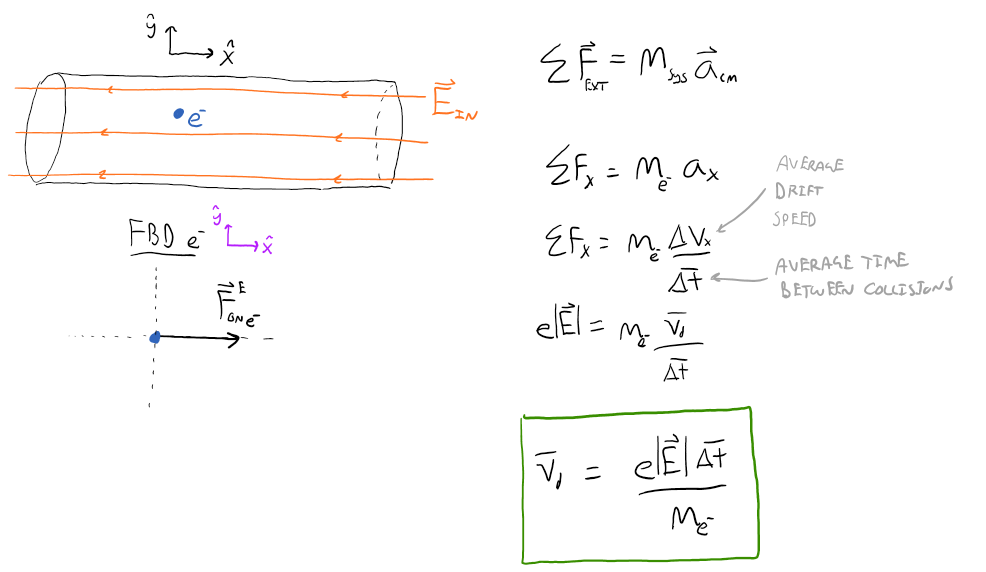
In the beginning we said that current is established in a conductor when free electrons have some net movement within that conductor. This was our motivation to look at how we get the free electrons to go through such motion. The analysis was a bit lengthy but is concluded with the mathematical model above relating the average drift speed of the free electrons, electric field strength, mass of electron, charge of electron, and average time between collisions of the electron and the ion core. We are finally at the point where we can introduce a more mathematical definition for current and begin to build a model based on that definition.

Microscopic model of current

With our classical Newtonian analysis of free electrons in electric fields out of the way, we will now construct a microscopic model of current. Let's first begin by defining current in the written description.

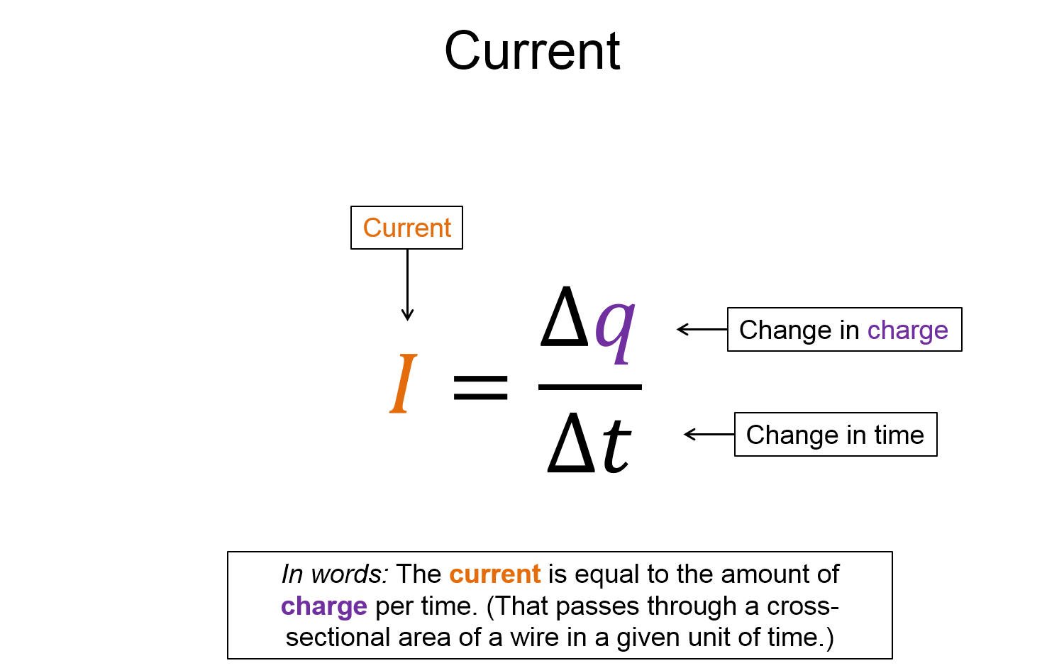
Current ≡ $I$ = The amount of charge that passes through a cross-sectional area of wire in a given unit of time. Mathematically we write current as:

$$I = \frac{\Delta q}{\Delta t}$$

Note that in SI units, current would be coulombs/second. We say that 1 coulomb/second is 1 Ampere, or "one amp". The conventional symbol we use for amp is "A".

With the written representation and the mathematical representation of current defined, let's look at a physical representation of how we could measure current. The image below shows a person with a stop watch counting the number of free electrons, each with average drift speed, that pass through a cross-sectional area of the wire. *Be careful, we are using A as the cross-sectional area, it is not representing the unit amp in the image below.

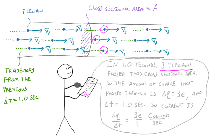
The above image also illustrates an important concept: conservation of charge. Here, conservation of charge states that the amount of charge that reaches the cross-sectional area in a given unit of time, must also leave that cross-sectional area in the same amount of time. This should make some intuitive sense, for example, if more charge enters the cross-sectional area than leaves it, then charge would build up on the cross-section. If charged built up on the cross-sectional area, then it would begin to repel the incoming charge thus reducing the current until it eventually stops. Basically, conservation of charge will ensure that our current is constant. As you might imagine, the image above is not representative of how we could actually measure current in the laboratory. Remember that even the thinnest piece of wire you can find has an Avogadro's number of ion cores and thus free electrons. So we should come up with a more clever way to measure the current.

Since it is basically impossible to count the large number of free electrons that pass through the cross-sectional area, perhaps we can work in terms of the density of free electrons. We will refer to this density as the charge carrier density and use the symbol "n". It should be noted that electrons don't necessarily have to be the charges that move to create current, thus whatever type of object that has charge and is moving is referred to as the charge carrier. However, in metals it is the free electrons, but in aqueous fluids it might be positive and/or negative ions. Back to charge carrier density, the image below shows how we would calculate it

It still might not be clear how finding a density would be easier, after all, it looks like we need to count the number of electrons in the unit volume V. With a little help from some chemistry terminology, we can use the definition of a mole, along with the mass density to write the charge carrier density in terms of easily measurable quantities. Below is the mathematical model for how we can calculate the charge carrier density assuming we know how many free electrons there are per atom in the type of conductor we are using.

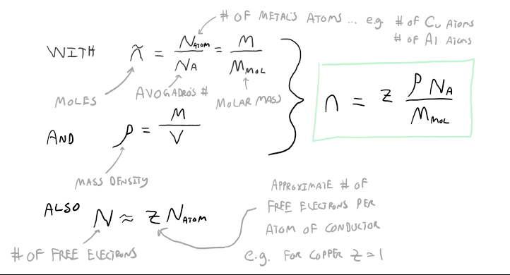
It would be a good exercise to work through the few steps of algebra to arrive at the mathematical model for charge carrier density shown above. Looking at the functional form of the charge carrier density reveals some important features. First, notice that it contains mass density and molar mass, both of which are relatively easy to calculate for a metal. Second, Avogadro's number is a constant. Third, we need to approximate the number of free electrons per atom which is another relatively easy task if assume that the electrons in the outermost electron shell are the free electrons. Using this approximation, copper would have z = 1, aluminum would have z = 3, silver would have z = 1, etc… Finally, since the mass density, molar mass, and "z" number are all material properties, this means that the charge carrier density is a material property. As a side note, in general the charge carrier density is not a constant: for example, as you increase the temperature of a metal, the number of electrons on the outermost electron shell can change, thus the charge carrier density of the metal could change.

We took a bit of a tangent, by showing why the charge carrier density is a relatively easy material property to calculate, but we are finally ready to construct that clever way of mathematically modeling current. Remember the players in this game are: the fundamental charge of the charge carrier (q), the charge carrier density (n), the cross-sectional area of the wire (A), and the average drift speed ($\bar{v}_d$). With our definition of current as charge/time, we can arragne the quantities listed in the sentence before to construct such a unit as shown below

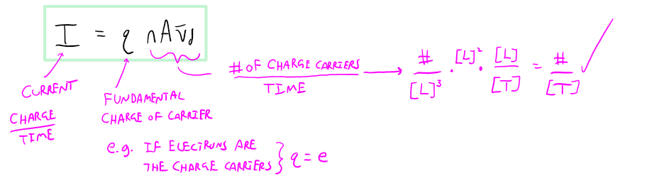
The above mathematical model is often referred to as the microscopic model of current. The functional relationships should make sense: if the charge carriers are moving faster their drift speed is larger and more charge will pass the cross-sectional area so more current; if the cross-sectional area is larger then there are more charges that pass through so that the current is larger; if there are more charge carriers per volume then more charge will pass the cross-sectional area so more current; finally, if the charge carriers have larger charge more charge will pass the cross-sectional area so more current.

Now is a good time to introduce a confusing convention: current flows in the direction that positive charges would flow, even if the charge carriers are negative. For example, look at the two images in this section, the free electrons are moving to the right, which is equivalent to saying a positive charge is moving to the left, thus current is flowing to the left in both images. This is just a convention that lasted for so long that we still use it. It takes some time to get used to, after all, the free electrons are moving to the right. Unfortunately it is the convention that everyone uses, physicists, engineers, biologists, chemists, etc.. so it is worth it to take a moment and let it sink in. Current flows in the direction that positive charges would flow, even if the charge carriers are negative.

Notice that we are talking about the direction of current, for example it is to the left in the images in this section. Although current has a magnitude and direction, it is not a vector. Remember scalars can be positive or negative, so we use the positive and negative to mathematically define the direction.

On the road to Ohm's law

In the above two sections, "force analysis of electrons navigating the conductors lattice" and "microscopic model of current", we basically constructed two independent ways of determining the drift speed of the charge carriers (e.g. free electrons in the previous examples). It is now natural to see what happens when we combine the two models. The algebra is shown below.

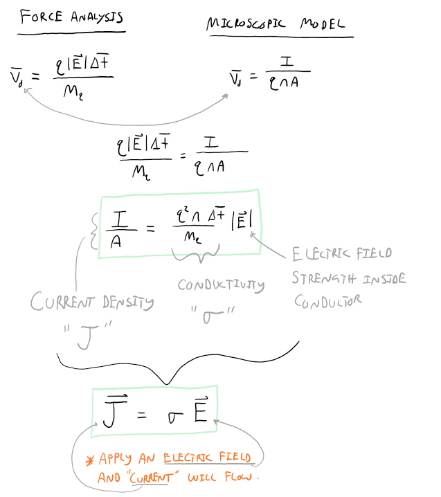
The above result is astonishing. First let's look at what the simplified version on the bottom is telling us; in short, "if you apply an electric field within the conductor, then you will establish a current". Congratulations, you've just constructed Ohm's law. If you have any previous physics or circuit analysis background, this might not be the familiar form of Ohm's law that you are used to, don’t worry we will get there soon, but it tells the same story. Before we construct the more familiar functional form of Ohm's law, let's take a closer look at the quantity labeled "σ" (i.e. the electrical conductivity, or conductivity for short). The first thing you should notice is that the conductivity is only dependent on material properties of the conductor: the charge of the charge carriers (q), the charge carrier density (n), the average time between collisions of the charge carriers and the ion cores ($\Delta \bar{t}$), and the mass of the charge carriers ($m_q$). This means that the conductivity is a material property. There are electrical handbooks that exist with the value of conductivity for every conductor commonly used. However, it turns out that the conductivity isn't quite a constant, rather it depends on certain features explained in the section below.

Conductivity (σ)

Mathematically conductivity is defined below

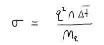
Where q is the charge of the charge carriers, n is the charge carrier density, ($\Delta \bar{t}$) is the average time between collisions of the carge carriers and the ion cores, and $m_q$ is the mass of the charge carriers. To get a better understanding of what role is plays, we need to look at Ohm's law as shown below

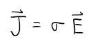
Notice it plays the role of a proportionality constant. For a constant electric field, if the conductivity increases, then you get more current/area (e.g. basically more current) to flow within a conductor. Thus, the larger the conductivity, the "easier" it is to get current to flow. Metals, which have lots of free electrons, have very large conductivities while insulators, which have very little free electrons, have very small conductivities. For example, copper's conductivity is about 6 x 10⁷ (s³·A²)/(kg·m²), and rubber is approximately 1 x 10^-14 (s³·A²)/(kg·m²). So to produce the same amount of current in rubber as in copper, you would need to apply an electric field roughly 21 orders of magnitude larger for the rubber sample than the copper sample.

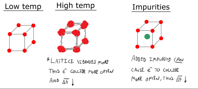
As previously mentioned, conductivity isn't quite a constant for any one material, it also has some external influences as shown below.

How can we affect conductivity?

• Charge carrier density (n) is slightly dependent on temperature as discussed previously. But we will consider it a constant over the normal temperature ranges encountered.
• The charge carrier mass ($m_q$) is constant.
• The charge of the charge carriers (q) is a constant.
• The average time between collisions of the free electrons and the ion cores ($\Delta \bar{t}$) is dependent on temperature and impurities.
  • How to affect($\Delta \bar{t}$)?
    • As temperature increases, the average time between collisions decreases and thus conductivity decreases.
    • Impurities can cause the average time between collisions to decrease and thus conductivity to decrease.
  • Below are images to help visualized why temperature and impurities typically decrease the average time between collisions.

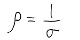
Resistivity

Recall that the conductivity of a material gives us an insight into how easily it is to establish a current, or in other words, how easily it is for the free charges to flow. If we take the inverse of conductivity we would get a quantity that gives us insight into how much the material resists the free charges desire to flow. This quantity is appropriately called, resistivity. We use the Greek letter rho "ρ" for resistivity. Mathematically resistivity is defined as the inverse of conductivity as shown below

Perhaps using resistivity in Ohm's law instead of conductivity will help illustrate its general meaning

Looking at the functional form of Ohm's law above, we see that for a constant electric field, the current density is inversely proportional to resistivity. Thus if the resistivity increases, the current density (e.g. the amount of current) decreases. This is why it's useful to think of resistivity as a measure of how much a material resists the flow of current. Recall that conductivity is a material property, thus resistivity is also a material property.

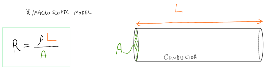
Resistance

We will finally exit the microscopic realm and enter the macroscopic in the section. Imagine you have a cylindrical piece of metal with length L and cross-sectional area A as shown below. As mentioned in the previous sections, this piece of metal has a unique conductivity (or resistivity). But as you would imagine, if you change the macroscopic dimensions of the metal, perhaps the ease of which the free electrons can travel from one side to the other will be affected. For example, if you increase the cross-sectional area, there is more room for the electrons to move about thus it is "easier" for the electrons to move along the length of the wire. On the other hand, if you increase the length of the metal, the free electrons have a further distance to travel to get to the other side, thus making it more challenging for them to move along the length of the wire. Using these ideas, we can construct a macroscopic term which gives us an insight into how much the macroscopic metal resists the flow of current. This new quantity is called resistance. We use the label "R" for resistance.

Finally…. Ohm's law in familiar form

We are finally in a position where we can construct the most familiar form of Ohm's law. Below are the algebraic steps. Basically, we combine our original definition of Ohm's law with the mathematical model for the change in electric potential in a uniform electric field.

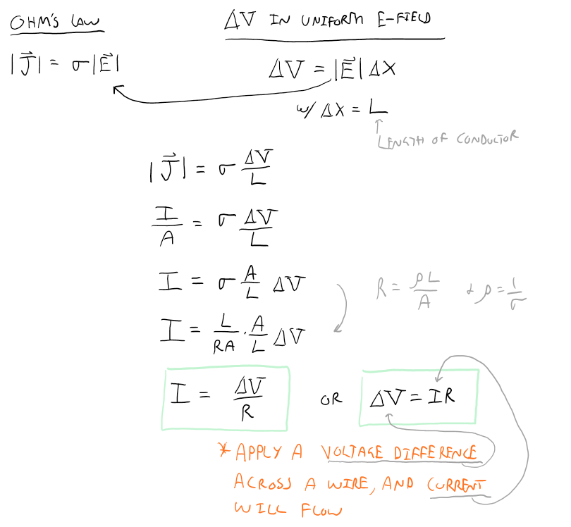
Congratulations, you just walked through a synthesis of multiple physics concepts and constructed the most familiar form of Ohm's law. Notice now the similarities between this new version and the previous version, the both say the same thing but use a different interpretation. The first Ohm's law dealt with electric fields, while the familiar form uses electric potentials.

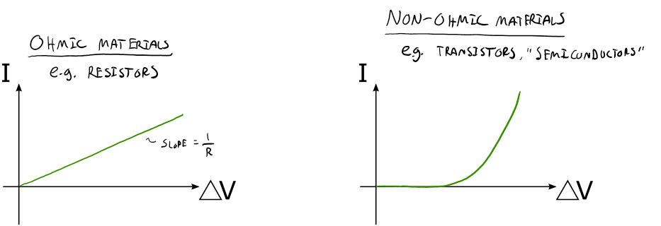
Don't let the "law" part of Ohm's law fool you. In fact, Ohm's "law" has a limited application since most materials do not obey Ohm's law. These materials that don't obey Ohm's law are cleverly called "non-ohmic". We are not out of luck though, certain circuit elements like resistors and lightbulbs can be modeled with Ohm's law under fairly wide ranges of conditions.

Let's get a graphical representation of devices that obey Ohm's law and those that don't. Below is a representation for each.

 

Key Equations and Infographics

---

 

---

 

Now, take a look at the pre-lecture reading and videos below.

OpenStax Section #.# | Title -- From Fundamentals

 

Openstax section on Electric Current covers the concepts for this section

 

Doc Schuster discusses the electric current and it's relation to the electric field among other things,

https://www.youtube.com/watch?v=8VZb9Khn9Mc

Pre-med Academy introduces the electric current.

https://www.youtube.com/watch?v=7-ChhK-P4aU

Other Resources

This link will take you to the repository of other content related resources .

 

For additional simulations on this subject, visit the simulations repository.

For additional demos involving this subject, visit the demo repository

Oh no, we haven't been able to write up a history overview for this topic. If you'd like to contribute, contact the director of BoxSand, KC Walsh (walshke@oregonstate.edu).

 

Resource Repository

Boundless online text covers different types of electric currents,

PPLATO is a complete resource with a lot of information, and several practice questions per subject. This webpage covers electric current and DC Circuits. We'll get to DC circuits after we deal with charge.

 

The Physics Classroom's section on electric current.

 

 

Isaac Physics' section on the electric current discusses current and charge

 

 

Other Resources

This link will take you to the repository of other content related resources .

 

 

 

 

Multiple Representations is the concept that a physical phenomena can be expressed in different ways.

Physical

Mathematical

Graphical

Descriptive

Experimental

 

(1) Mary has a copper wire with resistance $R_{cu} = 10 \Omega $. She wants to use an aluminum wire instead, but keep the same resistance. She has an aluminum wire with a radius $r = 0.25 cm$. What length of wire should Mary cut?

(2) A current with magnitude $I = 2 mA$ is running through a wire with an area $A = 2 cm^2$. If the density of charge carriers is $n = 100 $ electrons per meter cubed, what is the drift velocity of the electrons in the wire?

Short foundation building questions, often used as clicker questions, can be found in the clicker questions repository for this subject.

---

 

BoxSand practice problems

BoxSand's multiple select problems

BoxSand's quantitative problems

Recommended example practice problems 

• Electric Current, Website Link

For additional practice problems and worked examples, visit the link below. If you've found example problems that you've used please help us out and submit them to the student contributed content section.