Welcome to physics! This is the first lecture page for the course, it will review math used throughout and help to familiarize you with the way the content will be presented in the future. One of these pages is available for each lecture (take a look at the menu on the right! They look like "Lecture # | Topic"), with PH201 spanning Review and Vectors up to Energy. Each has a short trailer video for the topic, some reading, videos, ands supplementary resources. Even though it's Week Zero, try to spend some time here to make sure your math skills are up to snuff, as these topics and techniques will be used throughout the course!
Now, take a look at this short introduction to classical physics
Pre-lecture Study Resources
Read the BoxSand Introduction and watch the pre-lecture videos before doing the pre-lecture homework or attending class. If you have time, or would like more preparation, please read the OpenStax textbook and/or try the fundamental examples provided below.
BoxSand Introduction
General Review | Review
Significant Figures
Example: 37.12 meters has 4 significant figures if measured at centimeter scale. For our class, the general rule is to keep 4 significant figures throughout your calculations, or 5 for exponentials and logarithms. Your answer should use 3 significant figures.
Scientific Notation
Example: Speed of light in a vacuum $c = 299,792,458 m/s$ (not scientific notation), or approximately $3.00*10^8 m/s$ (scientific notation). Use the commutative property of multiplication to carry out calculations in scientific notation, for example:
Find the distance light travels in 1.2 pico seconds.
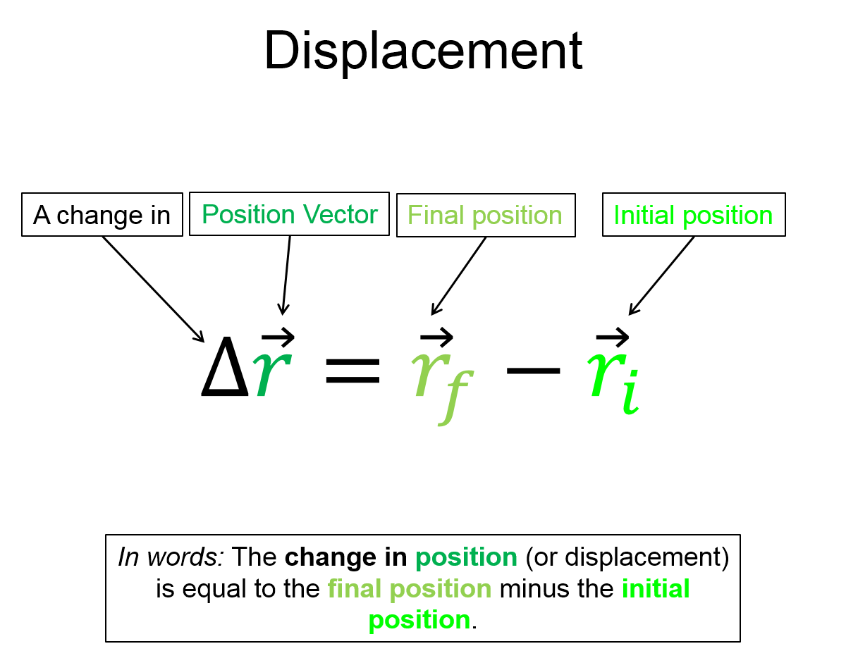
$c$ is the speed of light in a vacuum, and let $\Delta t$ represent the change in time. |$\Delta \overrightarrow{r}$| will represent the distance travelled, which you will see more of in Kinematics. Start out by representing the situation symbolically:
$$|\Delta \overrightarrow{r}| = |\vec{v}|\Delta t = (3.00*10^8 m/s)(1.2*10^{-12}s)$$
Now use the commutative property to switch the exponents:
$$= 3.00*1.2*10^8*10^{-12}m$$
$$=3.6*10^{-4}m$$.
Dimensions and Dimensional Analysis
Don't compare apples and oranges! That is, don't add, subtract, or equate objects with different dimensions. But you can (and will!) multiply and divide them.
Dimensions ([D]) are fundamental quantities like time, length, and mass. Dimensions are written with brackets, with time [T], length [L], and mass [M]. Other quantities in the study of the motion can be decomposed into time, length and mass, for example:
$$Speed = \frac{Length}{Time} = \frac{[L]}{[T]}$$
Apples $\neq$ Oranges $\to$ [A] $\neq$ [B]
To Reiterate, DO NOT and quantities with different dimensions!
Example:
$$\Delta x = v_{ix} + \frac{1}{2}a_{ix}\Delta t^2$$ (You'll see a lot more of this equation in kinematics. For now, just worry about the dimensions involved.)
$$[L] = \frac{[L]}{[T]}[T] + [?][T]^2$$
So, the dimensions of $[?]$ must be $\frac{[L]}{[T]^2}$ to even out. Overall $\frac{1}{2}a_{ix}\Delta t^2$ has dimensions of $[L]$
Units
In this class, we will default to SI (International System of Units), which are derived from dimensions. SI units are sometimes calles MKS (meters, kilograms, seconds). Here's a nice tabulation of SI units:
| Symbol | Name | Dimension |
| s | second | time |
| m | meter | length |
| kg | kilogram | mass |
| A | ampere | electric current |
| K | kelvin | temperature |
| mol | mole | amount of substance |
| cd | candela | luminous intensity |
Here's an example that uses Newton's second law $\Sigma \overrightarrow{F} = m\overrightarrow{a}$, which you'll see in Forces. Let's determine the units of $\overrightarrow{F}$ by looking at dimensions:
$$\Sigma \overrightarrow{F} = m\overrightarrow{a} \to [M]\frac{[L]}{[T]^2}$$ So $N$ has units of $\frac{kg*m}{s^2}$.
Conversions
Easy (No Powers)
Let's convert 100 feet per second to ? kilometers per day:
| 100 |
0.3048 |
60 |
60 |
24 |
1 km |
| 1 |
1 |
1 |
1 |
1 day | 1000 |
= 2633 km/day
Less Easy (Powers)
Now, what if we go from $10 m^3 \to cm^3$? There are 100 cm per 1 meter, so use that to "cancel out" the $m^3$:
| 10 $m^3$ | 100 cm | 100 cm | 100 cm |
| 1 m | 1 m | 1 m |
=
| 10 |
[100 cm]$^3$ |
| [1 |
= $10*10^6 cm^3$
Orders of Magnitude
Orders of Magnitude basically corresponds to counting zeros. More concretely, the powers of 10. For example, how many orders of magnitude larger is 1000 than 1? Well, count the zeros (or powers of 10). 1000 has 3 more zeros, so it is 3 orders of magnitude larger.
We have focused so much on creating introductions to the physics content we haven't had time to create text that reviews algebra and other prerequisite knowledge. We do however have good videos on what you'll need to know starting this class. Check them out below in the drop down called BoxSand Videos.
BoxSand Videos
Required Videos
*Note: there will usually not be this many pre-lecture videos
Unit Conversion - No Powers (4 min)
Unit Conversion - Powers (4 min)
Proportional Reasoning (5 min)
Suggested Supplemental Videos
none
OpenStax Reading
OpenStax is a great, free online textbook that we will reference throughout this site. The first chapter introduces the topic of physics, explains physical quantities and units, discusses precision, and covers approximations. Check it out if you prefer a traditional textbook presentation of content.
![]()
Post-Lecture Study Resources
Use the supplemental resources below to support your post-lecture study.
Practice Problems
A great way to prepare for the math requirement of this course is to work through the Algebra Review worksheet below.
Algebra Review Worksheet ======> Click HERE
Algebra Review Solutions ======> Click HERE
Additional Boxsand Study Resources
Additional BoxSand Study Resources
Learning Objectives
Summary
The first objective is to review prerequisite mathematical knowledge. The second is to introduce sense-making, which lies at the interface between problem solving and conceptual reasoning. Notable sense-making tools include: dimensional analysis, order of magnitude estimations, specials cases, and proportional reasoning.
Atomistic Goals
Students will be able to...
- Apply a working definition of answering with three significant figures.
- Show that they must keep more than the number significant figures they intend to answer with during intermediate calculations.
- Recognize that a complete algebraic solution reduces the error caused by significant figures of intermediate calculations.
- Convert a number into scientific notation.
- Perform mathematical operations using scientific notation.
- Use commutative property of algebra, and scientific notation, to perform basic calculations to an order of magnitude in their head.
- Identify the dimensions of physical quantities.
- Perform dimensional analysis on derived expressions.
- Know the SI units for physical quantities.
- Differentiate between dimensional analysis and unit analysis.
- Differentiate between fundamental and derived units.
- Convert between units.
- Differentiate between order of magnitude and "times as much".
- Perform back of the envelope estimations.
- Identify which quantities are changing and which are static, including numeric coefficients.
- Perform proportional reasoning on single variables raised to the first power.
- Perform proportional reasoning on single variables raised to a power other than one.
- Perform proportional reasoning on relationships involving more than one variable changing.
- Differentiate between sin(x) and cos(x).
- Recognize symmetries, like complementary angles, to simplify analysis.
- SOHCAHTOA.
- Apply the Laws of Sines and Cosines.
- Perform basic algebraic manipulations on equations to isolate a desired quantity or quantities.
- Appreciate the value of keeping equations symbolic throughout the algebraic manipulation.
- Solve N equations with N unknowns, by finding the value of an unknown from one equation and plugging that value into another equation.
- Solve N equations with N unknowns where the set has to be solved simultaneously.
- Translate between the descriptive (words) and the mathematical representation.
- Recognize the graphical features of these basic functions: y=x, y=x^2, y=x^3, y=constant, y=1/x, y=1/x^2, y=sqrt(x), y=sin(x), y=cos(x), for both positive and negative values of x.
- Recognize the graphical features of these basic functions: y=-x, y=-x^2, y=-x^3, y=-constant, y=-1/x, y=-1/x^2, y=-sqrt(x), y=-sin(x), y=-cos(x), for both positive and negative values of x.
- Check the sign of their quantities makes sense.
- Check the dimensionality and units of their quantities makes sense.
- Check the order of magnitude of their quantities makes sense.
- Check the behavior of a derived equation makes sense, e.g. proportional reasoning.
- Check the behavior of a derived equation in limiting (special) cases makes sense, e.g. as x goes to 90 degrees in sin(x).
- Check derived equations, functions, or values, are self-consistent, e.g. check that the slope of a derived position plot matches the values of the given velocity plot.
- Compare given or derived quantities with known values.
- Compare the relative magnitude of two related quantities
Problem Solving Guide
Use the Tips and Tricks below to support your post-lecture study.
Assumptions
- Given equations all work dimensionally, at any point, an equation can be evaluated in this way.
- All mathematical artifacts have physical meaning and interpretations in science. Compare previously known mathematical equations, units, and physical situations to previously understood ones to gain new insights!
- Many problem solving strategies are similiar, take a moment upon finishing a problem to draw a big picture about what you did in each step and connect it all together (you WILL see that picture again, somewhere down the line!).
Algorithm
1. Read and re-read the whole problem carefully.
2. Visualize the scenario. Mentally try to understand what the object is doing.
a. Motion diagrams are a great tool here for visual cues as to what the motion of an object looks like.
3. Draw a physical representation of the scenario; including vector diagrams
4. Define a coordinate system; place the origin on the physical representation where you want the zero location of the x and y components of position.
5. Identify and write down the knowns and unknowns.
6. Write out the mathematical representation for the physical representation you drew in step (3).
7. Carry out the algebraic process of solving the equation(s).
a. If simple, desired unknown can be directly solved for.
b. May have to solve for intermediate unknown to solve for desired known.
c. May have to solve multiple equations and multiple unknowns.
d. May have to refer to the geometry to create another equation.
8. Evaluate your answer, make sure units are correct and the results are within reason.
Misconceptions & Mistakes
OP Ed from former BoxSand content manager
"Physics has a different set of expectations than most other disciplines. We want to trin you to think critically and solve problems you do NOT know how to solve when you start them. This means we frequently need to throw you off an intellectual cliff and ask you to flap your arms for a while before relizing we gave you a parachute (and we always do!). This can be very frustrating for many students and can even seem cruel. However, the pay off of making you into an independant problem solver who can look at the natural world and truly make new insights and discoveries is too great to let some discomfort get in the way. Learning how to think is the goal, not answering individual questions correctly.
Oftentimes, more progress can be maden from failing to get a question correct, than from nailing it on the first go. We expect you to fail at first. We expect you to not get it right immediately. We want that. Do not let yourself think you're making real mistakes here. This is the scientific process in action. Just as it took 1000 tries at making a working lightbulb before getting it right and professional scientists plug away at a theory or experiement and make hundreds of "mistakes" for years before making the discoveries that their careers are definied on and their admired for. You too, need to make "mistakes" in order to learn.
Fail faster. Jump into problems half-cocked, be brave and go with your gut and what you already know, especially in lectures and homeworks where the price of making a "mistake" is very low. Don't let questions linger and ideas go untested long enough for you to still have reservations about them when its test time. Fail over and over again until you've learned how to make it work by then. Honestly, the best advice one can give is to fail faster!
Physics is primarily based on mathematical problem solving. It is okay to not feel comfortable doing math, but dreading it, saying you hate it, and letting the frustration of making mistakes get to you is a self-fulfilling prophacy, where you'll continue to dread and be frustrated by it. By the end of this course, you'll likely be better at alegbra and the math that you've already learned than you ever thought you could be, just stick to it
Respect powers and scientific notation, often the number of digits and significant figures can be truncated or approximated, but any *10^x is the most important part of the number. A tiny difference there can change an answer from being extrodinarily small, to enormously large.
Do not skip the sensemaking and conceptual questions when you're doing problems. The greatest thing this course can teach you is to be inquisitive and develop the skill set to answer questions you DON'T know the answer to. This is the real reason you're taking this course when you future career likely involves little to no application of the physical laws you'll learn here."
Pro Tips
1. Always check to see if your answer seems reasonable. What is reasonable? Well if you were solving for your friend Derrick's height and you got roughly the length of a skyscraper, you probably made a "mistake."
2. Check the units of your answer and the type of mathematical object your answer is, this will often be the first line of defense when you think something is amiss, and is ALWAYS a viable strategy.
3. For a complicated problem, ask yourself what the characteristics of your answer should be at the end, the units, the type, the order of magnitude. Will it be approximate? Should it be a value you already know? Will it be in a certain direction? What are the things it definitely should NOT be? All these questions will keep you engauged and invested in the process, will make you better at solving future problems, and lead to a lot of satisfaction when your intuition nails it!
4. Take note of the way we solve problems in class, especially in this review section. There are a million ways to do a multi-step unit conversion, but there are only a few that really show fully what you're doing and allow you to catch your mistakes, for instance. Listen to motivational questions you professor, TA, or LA asks when solving problems, they'll give you the real insight into how to solve these problems, more so than just memorizing equations that are useful and particular common situations. Learning how to think is the goal, not answering the question.
Multiple Representations
Multiple Representations is the concept that a physical phenomena can be expressed in different ways.
Physical
Drawing a picture of a physical situation is an amazing tool for understanding a problem. Even with limited artistic skills, it is so powerful that often how to solve the problem can come about just by drawing a picture.

Mathematical
Graphical
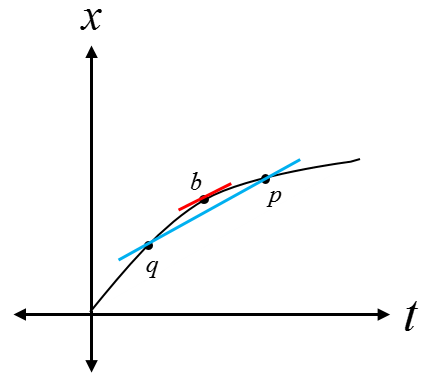
Below is a graph with position on the vertical axis and time on the horizontal. The curve shows a tangent line, or slope, representing in instantaneous velocity at one point. There is also a representation of the average slope and thus velocity between two points.
Descriptive
Experimental
We could go out to an ordinary city block and time how long it takes to walk from one corner of the block to the exact opposite corner. In this way, we could walk around the outside of the block and measure the distance traveled on foot around the block. Each side of the block would represent a position vector. From the mathematical representation section we would certainly know what to do with the rest information. Therefore, we can easily calculate the the average velocity.